Commercial use of this content is strictly prohibited. For more details on licensing policy, please visit the About page.
1. Vector Algebra
We will neglect very simple operations.
1.1 Triple Products:
1.2 Nabla Operator:
For a unit vector,
differentiation means how changes
as increases by an infinitesimal amount.
That is
Descartes Coordinate:
Spherical Coordinate:
And similarly for others.
Based on these tables, we can derive
gradient:
divergence:
To recap:
Gradient:
Divergence:
Curl:
Laplace:
1.3 Properties of Nabla Operators
Pf.
Since is analytic,
mixed parital derivative is equal.
Hence .
Pf.
Pf. Consider only one component (others are cylic).
Same for other components and join them together, proven
Pf. Consider only one component (others are cylic).
Same for other components and join them together, proven
Pf.
We have a triple product formula: .
Replace these vectors with and .
We have to explain the .
In this term you should not regard as a common vector and this is not a common numerical product.
Instead, is an operator acting on scalar .
With the operator understanding,
it will be easy to interpret why it becomes a gradient operator instead of a common product.
Differential operators require a function to act upon. The nabla operator always acts on the function to its right.
Pf.
Like this process:
The same,
Pf.
Because
then
Separately simplify the four terms:
Finally
Pf.
Similarly for .
Finally remove all and join results from and .
The formula will be proven.
Please note that the here is a dyadic tensor, not gradient.
Pf.
Pf.
Pf.
The components
Take divergence
Join them together, then
1.4 Dyadic Tensor
This is in fact tensor product. The final space is
The result is a 2-order tensor.
To interpret in components:
1.5 Levi-Civita Symbol
Then
1.6 Two Theorems
Theorem: If . then ,
Pf.
Suppose .
since , but .
Then for . 2 terms .
.
Theorem: If , then . .
Pf.
1.7 Application Examples
We offer some application examples here:
since
Then
(dyadic)
Since
Then
(dyadic)
Since then
2. Static Electric Field
2.1 Field and Potential
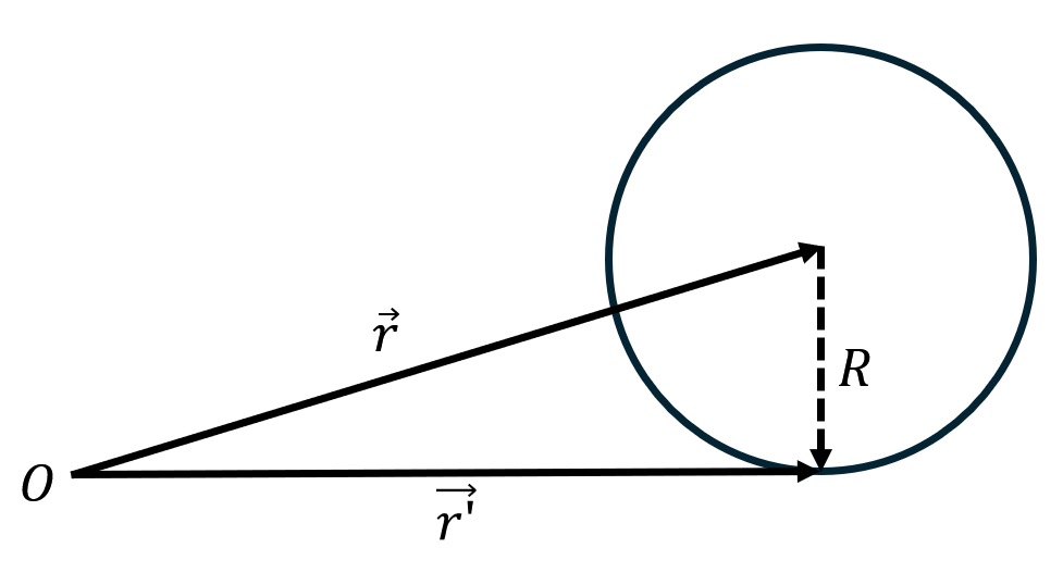
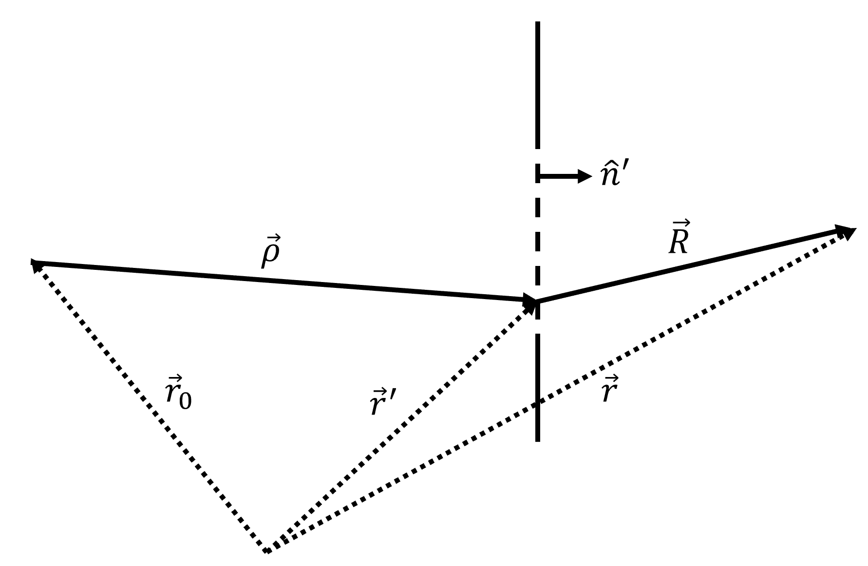
Note that is the absolute position of the measuring point, while is the position of the charges.
The formula above can be written in a compact form.
where
is defined as electric potential, which is a scalar potential field.
Note that the does not operate , for operates space. For a small field
is a constant vector (fixed charge).
Next we can calculate the curl and divergence
Take an arbitrary volume including .
At , , but the integral is finite. Hence .
Finally we get
From the derivations above, we can get some important conclusions.
Poisson’s Equation for static field:
Static electric field has a source but no curl.
Further, there’s Earnshaw’s law.
Earnshaw’s law: Point charge cannot be in stable equilibrium in static electric field.
Pf. stable equilibrium .
However , there’s a conflict.
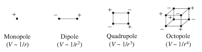
2.2 Multipole Expansion
When you’re very far away from a localized charge distribution, if , it can be approximated as a point charge. But if , to make things more precise, the charge distribution should be expanded as multipole.
Different Multipoles
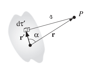
We now deduce the potential of multipoles. At certain point , the potential is given by
Using the law of cosines.
Define , then .
Field of a Charge Distribution
Apply Taylor expansion
Plug into the expansion,
Surprisingly, the coefficient of the terms are Legendre polynomial. We conclude that
The terms in the expansion above indicate the contributions of multipoles.
term is the monopole contribution. term is dipole, quadrupole, octopole, etc.
Ordinarily, the expansion is dominated by monopole, which is just a point charge.
If , the dominant term will be the dipole,
We define
as the dipole moment. The dipole contribution simplifies to
Generally, if you move the origin of the coordinate, will also change
The field of a dipole is
Also, we can extract the contribution of quadrupoles.
The two integrations can be combined into one term.
The quadrupole moment tensor is defined as
Obviously , hence , this is a symmetric tensor.
It’s easy to verify to be traceless.
Further, to get a more compact form, expand with a more compact form of Taylor expansion.
In static potential
The contribution of quadrupole
For the operator,
Plug this term into .
where
The electric field produced by a quadrupole is:
Consider .
First calculate gradient of quadratic form
Then
If a quadrupole is placed in the external electrical field , the energy should be
The monopole (total charge) and dipole of a quadrupole are both 0. Hence there’s only one term left.
Recall the potential expansion with Legendre polynomial:
The Legendre polynomial can be further expanded with spherical harmonics:
Plug the expansion into the potential and reassign them:
And multipoles can be defined:
is the elements of -poles tensor .
2.3 Uniqueness Theorem of Static Electric Field
Suppose a static system is composed by multiple uniform medium or conductor areas.
We have known the charge distribution ,
total charge or potential ,
and potential of boundary or its derivative in normal direction ,
then the field is unique.
This is the unique theorem.
Pf.
Suppose there are two potentials: , .
Consider two area in neighbor.
We have:
and
Define a differential potential
Then the differential potential satisfies
Consider the energy contained by the differential potential:
In the mean time
The second term vanishes because of the Possion equation.
Then
Now consider two types of boundary conditions.
If is given, then on the boundary,
hence ;
If is given, then on the boundary,
hence .
Then the theorem is proven.
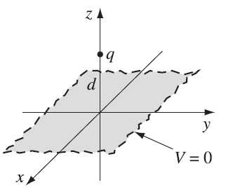
2.4 Method of Image
Suppose a point charge is placed over an infinite large, grounded plane.
Initial Configuration
The system satisfies two conditions:
These conditions in fact give the boundary condition. Based on the uniqueness theorem, there’s only one solution if satisfies the boundary conditions, regardless of the charge distribution.
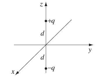
To simplify, another configuration can reach the same boundary condition.
New Configuration
Another at , and no plane. This charge is called image charge. In this configuration potential at is
This is the same as the configuration with plane.
It’s different at but no one cares.
Such potential is a combined contribution of both charge and induced charge .
Induced charge density on the plane is
The force is
Energy in this system
To recap, the essence of image method is the uniqueness theorem.
There’s another example.
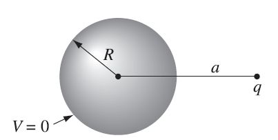
Sphere to Apply Image Charge
We try to use to replace the induced charge on the sphere.
To satisfy boundary condition , the image charge must be
Since , it must be a constant, must also be constant.
We can let
You can definitely take other values, but such value matches the intuition.
2.5 Green Function Method
This method performs better than image method in practice.
Consider general problem,
potential satisfies Poisson equation
To solve this equation,
we make some preparations first.
Giving two equations:
where is an arbitrarily chosen assistance function.
The two equations are called Green's first formula,
which can be deduced by Gauss formula
Further, subtract the two Green's first formulas:
This is called Green's second formula.
Choose
We have
then
Reassign it, we get Poisson formula
But choosing this assistance function has a drawback:
Look at the second and the third term,
if we want to know the total potential,
we must know the potential and its gradient on the boundary,
but in most cases we only know one of them.
Choose
Plug into the Green's second function
We have
If the boundary condition
is given, then
is a necessary condition for the solvability of Poisson function. If this condition is not satisfied, you cannot find a potential satisfying all conditions provided. The system does not exist.
Another important preparation is the mean value theorem. Consider a spherical surface
The potential at the center is
This result indicates mean value theorem. The potential in the center equals to the mean potential on the surface of the sphere.
Now it’s time to figure out some dominant problems.
Given Poisson function and boundary condition.
Take assistance function satisfying
Plug in and (gradient of on the surface is elliminated because )
Reassign it
Since is uniquly determined by the equation and boundary condition,
is also known.
So we do not need to give the gradient before the solution.
In fact the assistance function is called Green function.
Another type of boundary condition is giving the gradient (normal derivative).
Also, try to take assistance function satisfying
However,
this Green function will elliminate the solution,
since potential may have a solution only when
If ,
the potential is sovable if and only if the system is a vacuum that there is no charge.
To make it solvable in any cases,
the Green function is modified as
Plug in with this condition
Reassign it
where is the mean potential on the boundary.
3. Static Magnetic Field
3.1 Field and Potential
To show direction of current, we can define current density.
By charge conservation, in a closed volume,
Then
There’s an experimental law: Biot - Savart Law.
Biot - Savart Law: For 2 current elements and , the force between them is
And magnetic flux density
Further show in a compact form.
Similar to electric field, we can define a potential for magnetic field. But is a vector.
Further inspect .
For any function ,
Hence and
For the 1st term, because of
This term includes the entire space, so we can take a sphere with
Since at infinite far away points, the 1st term collapses to 0.
Meanwhile (no charge here), hence
For the 2nd term,
Finally,
3.2 Lorentz Force
Under all inertial systems, Lorentz force takes the same form.
For current
In general,
current density is propotional to the force per unit charge:
is the Lorentz force (mentioned in 2.3).
Plug in force,
Ordinarily the velocity of charges is sufficiently small and the term of magnetic field can be ignored.
where is called conductivity. This formula is called Ohm's law.
It may be confusing that we know the electrofield inside a conductor is 0. But there is current inside connecting wires made of metal, which seems to violates Ohm’s law. However, this conclusion is just an approximation. of a conductor is so large that only a very small field can drive large current. Hence in most cases, even if the charge are moving, the field inside can be ignored.
3.3 Multiple Expansion of Magnetic Fields
Similar to electro fields, the magnetic potential can also be expanded with a Legendre polynomials
What differs from electro expansion is that the monopole term
vanishes because .
This result indicates magnetic field has no monopole,
consistent with the prediction of
In the absence of any monopole contribution,
the dominant term is the dipole
From Stokes formula
Let , where is a constant vector.
Hence
Plug in ,
And finally get the potential of magnetic dipole
where magnetic dipole is defined as
The magnetic field by a magnetic dipole is
The proof above is a special case of a small, thin circle current.
In general cases,
is replaced by .
When a magnetic dipole is placed in external field,
the total force on it is
The first term is always zero since there is no current going into or out from the volume.
With higher order terms ignored,
Consider a 3-order tensor
and its divergence
Because the current on the surface is zero and ,
we have
Further for
By using the inverse form of
We can find
is a constant vector for a dipole.
So
The same, no current change results in .
By ,
the energy is also clear.
What necessary to clarify is that
magnetic effects are much weaker than electric effects.
Effect of magnetic dipoles is close to an electric quadrupole.
Therefore,
in most cases we only care about magnetic dipoles and ignore higher order effects
including magnetic quadrupole (whose influence is close to electric octopoles).
3.4 Uniqueness Theorem of Static Magnetic Field
Similar to electro, magnetic field also has uniqueness theorem.
Suppose there is constant current inside system ,
.
If current distribution, matter distribution and tangent component of or are given,
then in this system can be uniquly determined.
The proof is also similar.
Suppose , satisfies all conditions.
So it gives
Define differential quantity
obviously
We get the energy of differential field
The differential field contains no energy,
meaning everywhere.
Q.E.D.
4. Dynamic Field
4.1 Dynamic Electrical Field
Faraday discovers that the variation of will generate electromotive potential.
where is the magnetic flux.
We can deduce the differential form.
Remove , we have
4.2 Dynamic Magnetic Field
If we take variation of into consideration, we will find a conflict.
But take divergence to both sides.
This means , but it's not necessary in physics. Charge conservation indicates that
To cancel this conflict, we need a new term.
we have
then
4.3 Maxwell Equation in Vacuum
From the derivation above, we can summarize Maxwell’s equations:
Note that in the last integral form, the term
is often written as ,
where is the electric displacement field.
Similarly,
the magnetic field integral equation is sometimes expressed using the magnetic field intensity
instead of ,
where in a vacuum.
The image shows the latter using .
4.4 Completeness of Maxwell Equation
Completeness: Given the initial and boundary condition, the are uniquely determined.
Pf. Given initial condition.
boundary condition
Define
Then
According to Maxwell's Equation
Define
Then
With the initial condition, . Hence .
5. Fields in Matter
5.1 Polarization
A body with equal positive and negative charge \left(totally neutral\right) is called a dipole. When a dipole is placed in , it will be polarized.
The dipole has a dipole moment of:
is called polarizability, depending on the structure of the dipole.
If the distance between positive and negative charge is , then the moment can also be written as:
The direction of is from negative to positive.
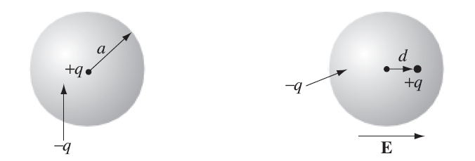
Take a polarized atom for example:
Polarized Atom
The field produced by negative charge is:
The positive remains stationary at equilibrium. Hence:
The polarizability is therefore:
For more complicated molecules, and may not be in the same direction. The is expanded as a tensor:
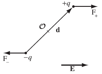
The torque by external field is:
In uniform field \left(or is very small\right):
Force on a Dipole
In non-uniform field, assume is very small. The total force is:
Then torque in non-uniform field:
And the energy of a dipole in field is \left(suppose at the center\right):
In uniform field:
5.2 Potential and Force of a Dipole
Now it comes to the field produced by a dipole.
The potential is:
and
Expand with Taylor series \left(for \right):
Ignore second-order term:
Then:
And electric field:
Example: Two interacting dipoles
Consider ,
5.3 Macroscopic Polarization
If an object contains many dipoles, is defined as the macroscope polarization:
The potential becomes:
where are the positions of field point and source respectively.
Reassign it:
The two terms are separately the potential produced by surface and volume charge. Hence
We did not take any free charge into consideration. All charge mentioned above is generated by polarization. They’re trapped in the object and cannot move freely. Such charge is called bounded charge.
5.4 Electric Displacement
We now take free charge into consideration.
By Gaussian law:
For convenience, define:
as the electric displacement, then Gaussian law is simplified:
In integral form:
For curl \left(ignore first\right):
For many substances, is proportional to :
Then:
In another view, permittivity changes with substance:
If the substance is not isotopic, the in different directions will change. Then will be expanded as a tensor:
The energy should be:
5.5 Magnetization
All magnetic phenomena are due to electric charges in motion. Like electric polarization, when a magnetic field is applied, a net alignment of magnetic dipoles (produced by polarized atom) occurs, then the medium is magnetized.
The magnetization is not always the same as external . Some are parallel (paramagnets), some are opposite (diamagnets). A few substances retain the magnetization even after the external field has been removed.
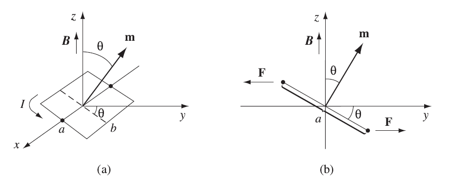
A magnetic dipole is a small current loop. The simplest example is a rectangular dipole.
Rectangular Magnetic Dipole
The torque in a uniform field in the z direction:
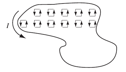
where is the normal vector of the dipole plane. For non-rectangular dipoles, we can fill the area with many rectangular sides.
Adjacent sides always have opposite current, so they cancel each other.
The sides next to the edge compose the original current loop. Then the torque can be expanded:
Non-rectangular Dipole
where , is the area.
For a current element in , force applied by field is:
Then for a macroscopic current:
For a current loop in uniform field:
In non-uniform field, suppose an infinitesimal circular wire ring of radius carrying a current :
Hence the energy:
Also, it comes to the dipole’s field and perturbation.
For current density :
In a dipole, :
Since :
And field:
5.6 Macroscopic Magnetization
For an object, define:
as the total magnetization. With , the potential of the object:
(due to formula )
The first term looks like the effect of volume:
The second term looks like the effect of surface:
Then:
The and are bounded current in the volume and surface, respectively.
Now it’s time to take free current into consideration:
By Ampere’s law:
Define:
as an auxiliary field, then:
In integral form:
The divergence:
only when ,
Similar as electric field, is always linear with :
Then:
is called permeability, and is called susceptibility.
When the substance is not isotropic, is always expanded as a tensor:
5.7 Maxwell Equation in Matter
We first list Maxwell equation in vacuum:
In matter,
and will be replaced with and .
According to chapter 5 and chapter 6,
Gaussian law is replaced with
Ampere law of loop is replaced with
5.8 Boundary Conditions
At the boundary of different substances, are not continuous.
Take a thin cylinder crossed by the boundary, with bottom area , infinitesimal height . According to Gaussian theorem:
and
And:
Take an Ampere loop with infinitesimal width , crossed by the boundary, length .
By Faraday’s theorem:
then
By Ampere’s law of loop:
This gives:
finally
6. Energy
6.1 Energy of Electric Field
First we research on discrete charge cases. For 2 charges, the work to move from far away to the position of \left(let to be the original point\right) is:
Bring more charge in.
The final work done should be the sum of all works.
Remove repeated terms.
when the discrete charges become continuous,
where is the field point and is the position of field source.
Apply Maxwell equation.
So
But , then
We're integrating over all space and at infinite far away .
So the first term
then
6.2 Energy of Magnetic Field
Suppose there're two loops at rest.
Run a stady current on loop 1,
it produces a magnetic field .
The Biot-Savart law gives
The magnetic field is proportional to current .
And so too is the flux of loop 2
is called the mutual inductance from loop 1 to loop 2.
Now plug in the magnetic potential:
Extract
We can find an amazing result:
the formula of is symmetric to and .
Hence, we can say
We then drop the subscripts and call both of them .
With the inductance,
according to Faraday's law,
magnetic field produced by loop 1 generates emf in loop 2:
Furthermore,
the current applied on loop 1 no longer generates electromotive force in loop 2,
but also generates in loop 1 itself.
Once more, it is also propotional to current:
This new coefficient is called self-inductance.
In an inductor, the electromotive force can be expressed with
Total work done per unit time is
So
Furthermore,
Hence
By Maxwell's equation,
So
Similarly, at infinite far away.
6.3 Poynting Theorem and Energy Conservation
Extract 2 equations from Maxwell equations:
Multiply as follows,
Subtract
Reassign this equation we get
We define
to be the energy density of EMF \left(Electromagnetic Field\right). And
to be the Poynting vector, representing the energy flow density.
The can also be assigned as follows
Hence Poynting’s theorem can also be expressed by .
is obviously the work done by Lorentz force. This equation indicates that
6.4 Energy Flow in Matter
When in matter, repeat the process above but with permittivity and permeability replaced:
Multiply as follows,
Subtract
Reassign this equation we get
This is the form of Poynting theorem.
The Poynting vector
and the energy density
7. Momentum
7.1 Maxwell’s Stress Tensor
We have known the force density
total force
We propose to express it with field alone.
To simplify , introduce Maxwell Stress Tensor
Hence
with component
The force density then simplified to
Integrate to get total force
7.2 Conservation of Momentum
We denote as mechanical momentum.
In an isolated space
This is a standard form of conservation function.
(variation of density = Flux out of the volume)
So the term
must also be a momentum.
It is carried by EMF. Define
as the density of EMF momentum.
Then we have
This equation is the momentum conservation law of EMF.
With representation of ,
we rewrite the equation into integral form in infinitesimal time
The left hand side is the total momentum variation in unit time,
including mechanical momentum and EM momentum.
Evidently,
the right hand side is therefore the total momentum flowing out from the region,
i.e., the momentum flux.
Thus, the tensor is also called momentum flow density tensor.
On the surface, momentum introduces force.
On an area, given its normal direction ,
recall the force integrand
On a unit area, assign as 1.
This vector is called stress vector,
representing the force on a unit area on the surface.
Besides, the normal component forms pressure
7.3 Angular Momentum
Based on momentum, introduce angular momentum,
8. Electromagnetic Waves (EMW)
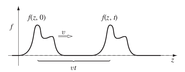
8.1 1D Waves
A wave is a disturbance of a continuous medium that propagates with a fixed shape at constant velocity. Suppose the displacement of points of the medium away from the equilibrium is . From the figure, we have:
Sketch of a 1D Wave
Let . We take the derivative of the function :
The second-order derivatives are:
The equations evidently yield the standard wave equation:
If we designate two parameters satisfying:
An eigen solution for the equation is:
where is the complex amplitude containing the initial phase. Since exponential functions form eigenstates, waves with any shape can be decomposed into components of exponential waves with different , but having the same velocity :
is allowed to extend into the negative region. With remaining positive, means . Obviously, the components correspond to waves that propagate toward the direction.
By fixing in the eigenwave , it is evident that the medium point returns to its initial state when provides a phase shift. Therefore, deducing the cycle (period) :
Similarly, fixing . When provides a phase shift, the point at behaves completely the same as . Such a length is called wavelength, denoted by :
The two fundamental parameters, and , are called wave number and angular frequency, respectively.
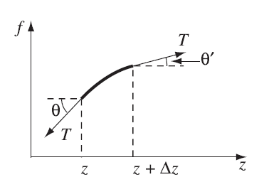
Different media have different abilities to carry waves. Suppose the resilience of medium points is provided by tension .
Tension in a Wave
We have:
Also, suppose the linear mass density is .
We then obtain the wave equation:
Compared to the standard equation, we have the wave velocity:
We can conclude that the medium type determines the wave velocity.
8.2 Polarization
In reality, 3D waves are more practical. In 3D space, the eigenwave is:
You can just join the directions together for they are independent.
3D waves have 2 types.
Waves whose displacement of medium points is perpendicular to the propagation direction is called a transverse wave. Waves whose displacement is parallel to the propagation direction is called a longitudinal wave.
For transverse waves in 3D, the displacement has 2 possible basis directions.
If the displacement is along :
Along :
The displacement can also oscillate along any direction in the plane. Suppose the vector is (with ):
8.3 EMW in Vacuum
In a vacuum, there are no free charges () or currents (). Maxwell's equations simplify to:
Taking the curl of the second equation, :
Using the vector identity . Since , we have:
On the other hand, substituting the fourth Maxwell equation, :
Equating the two results for , and similarly for , we obtain the wave equations:
Recalling the standard 3D wave equation , we compare it to the and equations to find the wave velocity:
In a vacuum, this velocity is denoted as the speed of light :
The eigenwave solution is:
Since the wave equation is deduced from Maxwell's equations, all solutions must satisfy Maxwell's equations. Applying and :
For a wave propagating in the -direction, this requires the -components to vanish:
Since the -components of and vanish, the EMW is a transverse wave. This simplest eigenwave is called a monochromatic planar wave.
Moreover, applying Faraday's law, , we get the relationship between the amplitudes in compact form:
There is nothing special about the -direction. In general, the monochromatic wave is:
where is along the direction of propagation.
The energy density is:
Substituting and into the expression:
Complex expressions cannot be measured directly; the magnitude is the amplitude and the argument is the phase. What is measured is the real part.
As the wave travels, it carries energy along with it. The energy flow density is represented by the Poynting vector:
For a monochromatic wave along the -direction:
The momentum density is:
Since the electric field varies so rapidly for light (a kind of EMW), we care about the time average(), analogous to the efficient value in alternative circuits.
Average energy density:
Average Poynting vector:
Average momentum density:
The average power per unit area is called intensity :
Momentum brings pressure. The radiation pressure is:
8.4 Diffraction
The fundamental method to solve diffraction problem is to solve wave function under given boundary conditions. Consider an arbitrary component of or , denoted as . satisfies wave function
For monochrome wave with frequency , . Define wave number . Plug in to get Helmholtz equation (at the source, as a boundary equation)
It may be confusing why prime appears suddenly. In fact satisfies Helmholtz equation anywhere without charge. But in diffraction problem, we treat the incident wave on the aperture as a source, accordingly to Huygens principle. Therefore the wave on the aperture serves as a boundary condition. We derive the wave in the entire space through Green function method. Now select a Green function, the spherical wave produced from a unit source at source point
where . It satisfies
Apply Green's second equation
Replace and with
then
We need for further calculation.
In optical view, , then .
Assume the incident wave is a spherical wave from ,
Similarly
Plug all into
This equation is called Kirchhoff equation.
Diffraction Configuration
At far positions, , . The integrand simplifies to
8.5 EMW in Matters
In linear matter, Maxwell equations become:
When there is no free charge and current, the equations collapse:
Then everything is the same as that in vacuum. The only difference is:
is called the index of refraction. Everything is the same after replacing , with , .
The energy density is:
The Poynting vector is:
The intensity is:
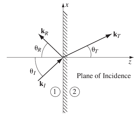
An interesting problem is the behavior on the boundary. According to the boundary condition:
Define Incident, reflection and transmission waves now.
Incident:
Reflection:
Transmission:
Behavior at the Boundary
At the boundary define , i.e., only components included. Then at any point , the 3 fields are:
Apply the tangent boundary condition:
This equation holds for any . Hence the exponentials must satisfy:
Incident and reflection wave share the same velocity, therefore . So:
We deduced the reflection law. Next, , .
All waves share the same . Then for incident and transmission wave:
We deduced the refraction law, also called Snell's law.
With exponential factors taken care of, they cancel. The tangent boundary conditions become:
Generally, the and are decomposed to and components. Relative to the incident plane, -polarization is defined as oscillating perpendicular, while -polarization is parallel.
For -polarization, the tangent electric field condition is:
The magnetic field condition is:
Substituting and :
Since :
Recap the system for -polarization:
For -polarization, the system of equations is:
Solve them separately.
The reflection () and transmission () coefficients are:
Recall Snell's law, it holds at any :
Experiments discover that under a certain , vanishes. Denote this angle as . We have:
Deduce like that:
Substitute from Snell's law:
The ratio for is:
This angle is called Brewster angle. In this case:
This means at this incident angle, reflection and transmission wave is perpendicular ().
Incident wave will force the particles in the secured medium (regarded as dipole) to oscillate.
-polarization waves cause oscillation inside the incident plane. However, dipoles do not release energy along the oscillation direction.
In the second medium, dipoles are driven by the transmission wave. When , the reflection direction coincides with the oscillation direction. Therefore, no energy is emitted.
The 4 coefficients are called Fresnel coefficients. For an arbitrarily polarized wave, we define:
Incident Electric Field:
Reflected Electric Field:
Energy reflection rate :
Transmitted Electric Field:
Energy transmission rate :
By energy conservation:
8.6 Absorption
Conductors usually absorb energy of EMW. There is no bounded current or charge. Free current is not zero:
The Maxwell equations change:
Moreover by continuity equation:
Solve :
Any initial charge dissipates. For a perfect conductor, . There is no accumulated charge. In this case:
The wave equation becomes:
Monochromatic wave and is still admitted, but the wave number is introduced as a complex number, where .
Generally:
The imaginary part results in an attenuation with space. The characteristic attenuation length, also called skin depth, is defined as:
At the boundary of a medium and a conductor:
For a non-perfect conductor, the process is very similar. We suppose the incident wave is perpendicular to the surface, therefore . By the tangent condition, with :
Incident:
Reflection:
Transmission:
We suppose the incident wave is perpendicular to the surface,
therefore .
By tangent condition,
with .
with .
Solving for coefficients:
Reflection coefficient :
Transmission coefficient :
The ratio determines the reflection/transmission property.
For a perfect conductor, , the skin depth . , .
Then , .
If (non-magnetic), then , .
is complex. .
8.7 Dispersion
Sometimes the speed of a wave depends on its frequency. This phenomenon is called dispersion, the supporting medium is called dispersive, which is a natural characteristic of the medium.
In a dispersive medium a wave composed by a range of frequencies change its shape.
One frequency represents a monochromatic wave, which travels with phase velocity
The wave packet as a whole travels with group velocity
Now we dive into the dispersion. We assume electrons are bounded at an equilibrium position by a quadratic potential.
The binding force is
Evidently the actual potential is , instead of . Here our goal is to describe the small oscillation of electrons. In fact, every potential can be expanded
At equilibrium, . Take potential at the equilibrium as reference, then .
Hence for small perturbation, .
Electrons are damped during motion.
is the damping coefficient. Furthermore external drives the oscillation.
Getting the motion equation
Solution
Oscillation of produces dipole . Suppose each molecule possesses electrons with natural frequency ( is the natural frequency of the medium).
molecules per unit volume. The total polarization
Polarizability is defined by
Hence
At this time dielectric constant is a complex constant, then reflection rate
is also a complex number. The wave number
Real part of contributes to the real part of , working as the original wave number, determining the wave length. Imaginary part of contributes to absorption. The attenuation term is .
The attenuation coefficient
The factor 2 is because .
With these relations derive relation of with
Separate Real and Imaginary part.
Generally, of visible light is far larger than . The absorption is very weak. In this region we can ignore .
Since , can be expanded.
Define
then
Absorb into .
This is called Cauchy's formula.
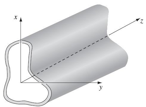
8.8 Guided Waves
Consider EMW confined to the interior of a hollow pipe. The hollow pipe is called wave guide. It is a perfect conductor, so inside , . The boundary conditions at the inner wall are
Wave Guide
The two equations above are constraints for EMW inside the hollow. Electro fields yield normal condition.
in the conductor is 0. To satisfy the conditions, free charge and current are induced on the inner wall. Suppose EMW
they satisfy
Solve them by components
When we operate on , it gives
Similarly for
Therefore we can replace the , operators with , to simplify.
The wave equations yield
In a wave guide, and cannot be zero simultaneously.
If
If
Raise them to second order derivative
They hold simultaneously only when , . However they're oscillatory.
Q.E.D.
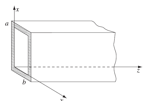
We take a rectangular wave guide. We let and
Rectangular Wave Guide
So
Divide by :
where
The solution is
because of .
requiring
plug in
Results in
Similarity for :
Then
Notice that 's spatial frequency is discrete, which is an inevitable result of periodic boundary condition. () forms modes of EMW in the wave guide.
At mode :
The wave number will become imaginary if
is called the cut-off frequency of the mode. Any component with frequency less than will be absorbed by the wave guide. The lowest frequency or is called dominant mode (depending on which is smaller).
In the derivation above we let , meaning is transverse. Such modes are denoted as . If we let , the derivation is completely the same and results in a set of completely different modes, denoted as .
When a monochromatic wave with frequency enters the wave guide, the energy is immediately reallocated to modes, including and . Only modes with can pass, while other modes are absorbed.
In a wave guide energy propagation is determined by Poynting vector
We only care about the propagation along -axis. We then decompose .
where are in plane. Extract magnitude of .
and forms a Hilbert space. Check whether the inner product of for different modes
can be prove whether different modes influence each other.
We prove it now. In modes.
Field in plane
Take inner product for 2 modes
Similarly
has the same conclusion. Then
We can say different modes are orthogonal.
Back to the monochromatic wave. With orthogonality, the should be decomposed by modes.
The coefficient is determined by:
We didn't consider incident angle, for the modes are results of reflection, refraction and so on. The angles have been encoded in the .
9. Radiation
9.1 Potential Formulation
From Maxwell's equations,
It can be written in the form without curl,
In terms of and , can be derived
Combined with
The field can be directly derived from potential . But for specific , is not unique. Suppose two sets of potential and ,
We assume they give the same , then
We can write as a gradient of some scalar,
then
The term in parentheses is therefore independent of position,
where depends only on time. We can absorb into , while no other effect caused.
Then
thus, any scalar function can change and get another set of potential which gives the same field . This transformation is called Gauge transformation.
There're two commonly used gauge called Coulomb Gauge and Lorentz Gauge, respectively.
the Coulomb Gauge, we pick
with this,
In Coulomb gauge the scalar potential is determined by the distribution of charge right now, which seems to be conflict to the relativistic limitation of propagation speed . To explain this, is not a measurable quantity, the measurable quantity is . However
When changes also changes, eliminating parts of variation of . Finally, propagates with speed . Under Coulomb gauge, is easy to calculate but is difficult. In Coulomb gauge, D.E. of is
In Lorentz gauge we pick
This is designed to simplify the equation of and . With this,
Meanwhile
becomes
We can notice and follows the same form.
These equations are called d'Alembert equations.
Lorentz force can be expressed in terms of potentials.
The derivative term of
is called the convective derivative of , and written as .
Then
The EMF inserts some extra terms for momentum and energy. We define canonical momentum
and velocity-dependent energy
9.2 Retarded Potential
Electro-magnetic effect propagates with speed . Thus, if an observer observed EM effects at field point , it is generated some time before at source point . The delayed time is
Then at time , at we observed effect at
The time is called retarded time. A natural generalization of potential is
These're called retarded potentials. Do they satisfy d'Alembert equations?
And
where
Take divergence
Thus
Electric potential satisfies d'Alembert equation. Similar for . Hence, retarded potential is a valid potential in Lorentz gauge.
Given retarded potentials
Evidently
and we've calculated gradient of . With
As for , we first find
Then
The two equations are called Jefimenko's equations.
When charges accelerate their fields transport energy out to infinity, called radiation. Suppose the source is localized near origin. The power passing through a closed surface is
EMW travels at the speed of . The energy leaves source at . Then,
9.3 Specific Radiation Fields
Alternative Current
Alternative current brings periodic current and charge
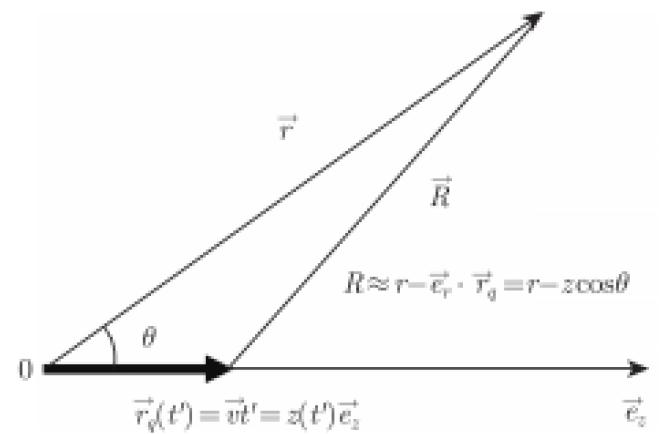
Plug in to retarded potential
where
By the definition of radiation, we should make . Then make an approximation.
Plug in the approximation.
Further expand
We derive and from Lorentz gauge.
Consider term of
Then
Then can be decomposed with orders.
The average Poynting vector on a period (like the effective value in AC current)
the power of radiation
Evidently, for , the integrand becomes 0. Thus, only term contributes to the radiation. Then the potential can be simplified.
The magnetic field
We neglect higher order terms in . Similarly we get scalar potential.
According to
and
then
Average energy flow density
And radiation power
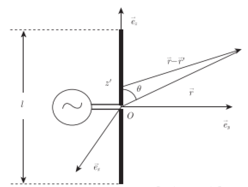
Thin, Straight Antenna
Suppose the length of the antenna is . Take the medium point as the origin. Varying current is input from the origin. The antenna is a good conductor.
Thin, Straight Antenna
Electro field inside the antenna is 0. On the surface,
Thus
Take derivate to time,
Since has only -component, Then
With Lorentz gauge,
we get
This is a wave equation. According to the relation between and , we can say
At , . Thus is a standing wave.
where . We then calculate radiation power.
where . When the antenna is small (), we approximate with .
The total power is
Radiation power increases rapidly with the increase of .
Antenna with is called half-wave antenna, with . Plug in,
The strongest direction of radiation can be determined by
We get is the strongest.
Multipoles
Suppose the size of system , where is the wavelength of EMW. Meanwhile . Under this condition we expand with .
The first corresponds to dipole radiation and the second term quadruple.
We check dipole first. We calculate
Integrate both sides.
The integrand equals to zero because on the surface. Thus,
Hence
Magnetic potential
Field
Poynting vector
then
Next we deal with quadruple. Consider the second term of
We focus on both terms. First inspect:
Then
Then
And
Take derivative over time,
The negative term
Then the second order potential,
is separated into quadruple contribution and magnetic dipole contribution. For quadruple,
For magnetic dipole,
10. Relativity in Electrodynamics
10.1 Special Theory
Maxwell equation predicts that light propagates in some medium. People used to think it is ether, an absolutely static, inertial reference frame. But Michelson-Morley experiment denied the existence of ether. To solve the conflict, Einstein raised to famous postulates.
The principle of relativity: The laws of physics apply in all inertial reference systems with the same form.
The universal speed of light: The speed of light in vaccum is the same for all inertial observers, regardless of the motion of the source.
The first term states that there is no absolute rest system. The second states that there’s no ether.
Now based on the two postulates, we derive the coordinate transformation rule in relativity, called Lorentz transformation. The transformation in classical mechanics is called Galileo's transformation.
Take two interial reference systems , . moves along positive axis at speed . Suppose , , , when the origin points and coincide, .
Suppose the transformation is linear. Then for any event
Since there's no relative motion in and direction,
The light signal starts at and . In two directions, two frames, the universal light speed separately yields:
Meanwhile, the origin of in moves at speed . The coordinate of in is
Combine all the equations, we rewrite them in matrix form.
Since ,
And
The same, negative light yields:
Combine the two
We also have , . Then
giving
We can rewrite the transformation in the form of a matrix
The transform should not scale or inverse the orientation, thus,
Now we can solve the coefficients. To simplify, we define two factors.
The results are:
The Lorentz transformation is thus
The inverse transformation should keep the form. Replace with and exchange coordinates
The we can derive velocity transformation
Inverse is
We consider that is also a dimension, thus the space become 4D. We denote coordinate in
and in
And Lorentz transformation read
With tensor notations, we can denote
where
is called Lorentz transformation matrix.
If the direction of the velocity changes, the Lorentz transformation matrix changes into a 3D version
where , , .
Now we define the inner product of 4D vectors. Suppose a light propagates in vaccum. In , it travels spatial distance
Since speed of light remains constant in all inertial reference frames, then
We rewrite
For a specific event, this equation holds in all inertial frames. It's natural to define space-time distance between two events
The assumption is successful, for it is the root of Lorentz transformation. Then a modulus of a 4D vector is defined as
And inner product is natural
The definition is good because it remains constant in Lorentz transformation
Modulus is a special case for the inner product. This means that spacetime interval remains constant under Lorentz transformation.
We have been using contravariant vectors. It’s necessary to introduce covariant vectors . If It’s the first time you hear about this, please check this link. Tensor Algebra.
Such a definition keeps the inner product
Introduce a metric
By definition, the metric tensor is therefore
called Minkowski metric. The spacetime space is called Minkowski space. Minkowski space is a pseudo-Euclidian space. With the metric tensor,
Since Minkowski space is not completely Euclidian, the inner product is not positive-definite. It can be positive (spatial terms dominate) or negative (temporal term dominates). We define displacement of two events
And its magnitude can be positive or negative. We further define
Where is the spacetime interval of event A and B. Recalled the postulate of universal speed of light, it also tells us that signals cannot propagate at speed exceeding . Now, if event B is caused by A, then they must be able to be connected by sub-lightspeed signals. Mathematically
This means
i.e.,
Thus, timelike events means causality between A and B is physically allowed (not necessarily). Similarly, if the interval is spacelike, causality is not allowed, the sequence of events may change after Lorentz transformation. Lightlike events must be connected with lightspeed when establishing causality. The signal must have zero mass. Lightlike is the limitation of causality.
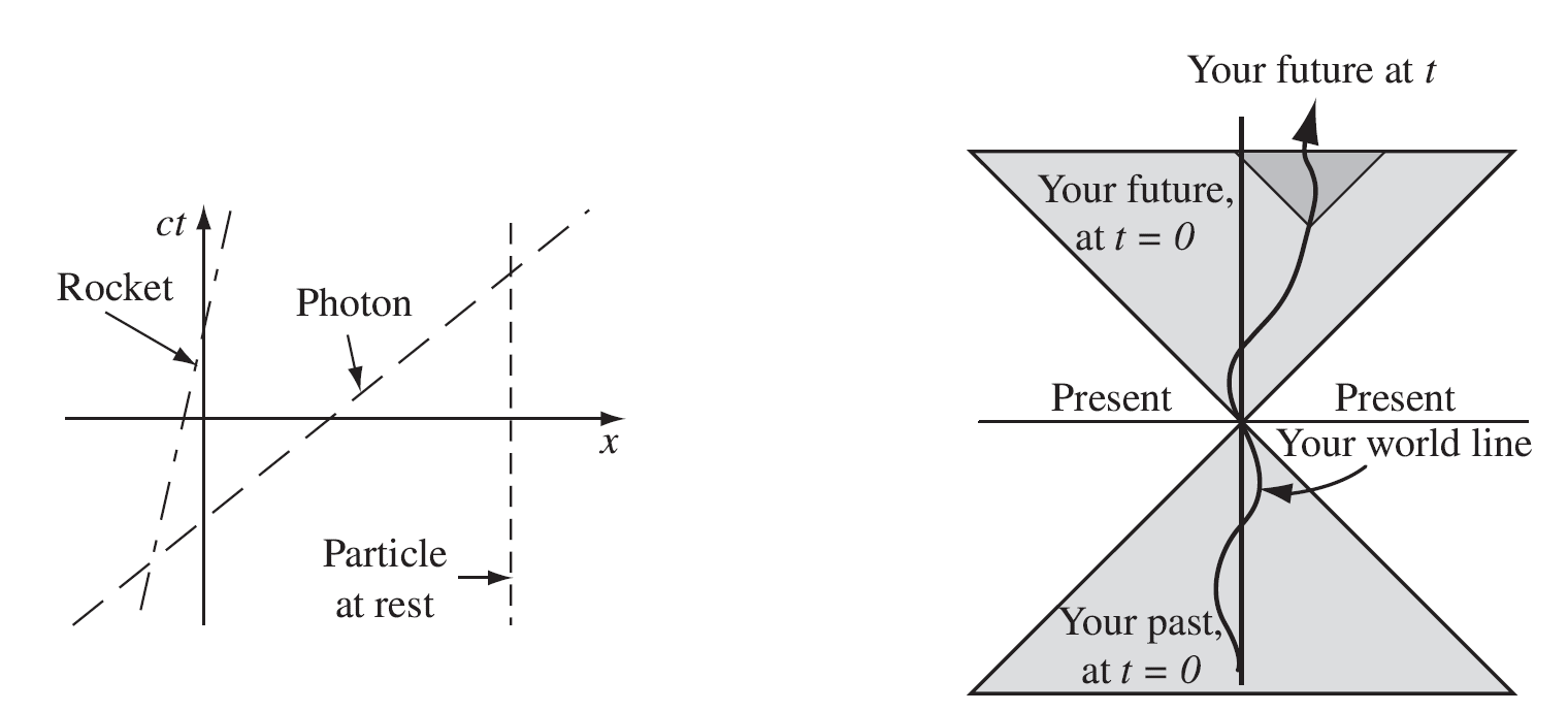
We can represent motion graphically by Minkowski diagrams. We plot spatial coordinate horizontally and time coordinate () vertically.
World Lines and Light Cone
The trajectory on a Minkowski diagram is called a world line. If a particle is at rest, its spatial coordinate remains constant with time flowing. Then its world line is vertical. Lightlike events occurs on , a straight line with slope . Since no particle can travel exceeding , so world lines with slope less than 1 are not allowed. Suppose you set out from the origin at . The two lightlike lines (positive motion) and (negative motion) defines your past and future allowed by physics.
The structure forms a cone geometrically, called light cone. If and are included, it will be a hypercone.
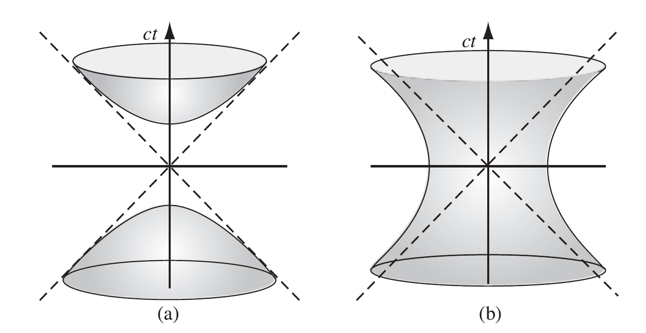
In the Minkowski diagram, we choose two events and calculate their spacetime interval. One of the event serves as reference. In the hypercone we assume at the two events occur at the same position (spacetime interval ). But in most cases they do not. At , they usually have an initial spacetime interval.
When , it means the displacement are spacelike. At , they occur as different positions, no causality allowed. Since , they occur at , respectively. The light cone is skewed out, turning to a hyperbola with the focus on space subspace (in 4D space, hyperboloid).
When , timelike. At , they occur at different time . The Minkowski diagram is also a hyperbola / hyperboloid, but the focus in on the time axis.
Hyperbola and Hyperboloid in Minkowski Diagram
In Minkowski space, Lorentz transformation is a pseudo-rotation. With metric,
This is equivalent to
In matrix form
Denote inverse matrix , satisfying
Since is pseudo-orthogonal, . Then
Then, for contravariant vector
for covariant vector
Reassign the index, we have
Now we inspect tensors under Lorentz transformation. We start out from a scalar which is obtained from contraction
under Lorentz transformation, should remain unchanged
Vectors are transformed:
Plug in
Eliminate and :
Then
But if is full contravariance, the condition become:
Plug in
Then
Further
10.2 Relativistic Mechanics
In Minkowski space, spacetime velocity is defined by
where is called the proper time, representing the time that the particle feels. (time in the frame moving together with the particle), which is a fixed parameter for a specific particle. Also, it means is a constant under Lorentz transformation. Then spacetime velocity is defined by
Apply Lorentz transformation matrix
Now there's an interesting conclusion. For any particles, the magnitude of spacetime velocity is a constant.
It indicates that in 4D Minkowski space, all particles "flow" along its world line at speed . If spatial velocity is not , velocity projection on time axis will be smaller, and the proper time slows down.
Now place an interial, static observer, whose velocity is
Minkowski space has orthonormal basis.
Of course we have other space basis vectors, but one is enough for our derivation. Suppose 3D spatial velocity in observer frame is
Define time dilation factor
In Minkowski space, the velocity projection on space subspace is not due to time dilation
Then
Combine
Apply magnitude condition
Finally
Then we know
This is the time dilation. Proper time is slower than time in reference frame (we call it "ordinary" time). Please pay attention to the subscript in the factor and do not confuse this with the factor introduced by the motion of the coordinate system at velocity . In following sections, we will call parameters in the moving frame () "proper" parameter and that in reference frame () "ordinary" parameter.
Besides time dilation, a moving ruler also shortened in the view of frame (reference event in Minkowski space). Consider a lever with fixed length . We want to measure the coordinate of both sides at the same time, thus, measuring must be completed by two events. In static frame , the world lines of sides of the lever are and , separately. Dynamic frame moves along at speed . We will measure the lever in and get the measured length .
In , we require two measuring events satisfy . Suppose in , the left event is , the right event is . Lorentz transformation gives
In , ,
Thus
Hence in , time difference of the two events is . In , 4D displacement is
Through Lorentz transformation, in
The second component is the desired length
Thus in , measured length is shorter than its fixed length.
To keep momentum conservation in all inertial frames, relativistic momentum is defined with proper velocity.
The temporal component is naturally
In quantum mechanics we have known that time translation invariance corresponds to energy conservation, and spatial translation invariance corresponds to momentum conservation.
In relativity, spacetime translation operates a vector and the conservation flow is also a 4D vector — . Its time component corresponds to time translation invariance, i.e., energy. The spatial component is then naturally momentum. But does not have energy dimension. So the energy is defined by
When the particle is stationary,
In motion, the extra energy is kinetic energy.
Like velocity, in Minkowski space the energy and momentum is always conserved.
Replace with , then
The force in Minkowski space is
The spatial force
is the mechanical force we'll measured in experiments, where is the relativistic momentum. The first term
represents the power delivered to the particle.
In relativity, the center of mass in classical mechanics is replaced by the center of energy.
and the total momentum is
10.3 Relativistic Electrodynamics
Maxwell equations have satisfied relativity under Lorentz transformation. To prove, we need to rewrite Maxwell equation in the form of a tensor. Config a frame , and another frame moves along positive axis of at speed . We have Lorentz transformation
According to the rule of chain, we have
In ,
Transform derivates into
Charge conservation holds in all inertial frames. Assume transformation is linear.
In
Plug in and compare corresponding coefficients,
Indicating that satisfies Lorentz transformation. If we construct 4D current density
It satisfies
Charge conservation turns to
The is 4D divergence of . So it states that current density is divergenceless in 4D.
With , we can then define 4D potential
We want a tensor (2 fields) for fields now. We know in classical theory and are composed by derivates of and . In 4D space, it's natural to use 4D derivate.
Gauge invariance is required. The field tensor should remain unchanged under gauge transformation . However, is not gauge invariant. But anti-symmetric quantity
is gauge invariant because . With this definition, components are easy.
For
For , spatial components
In expanded form
To express physical laws simply, we construct a dual tensor of . Substitute with and with .
With this tensor, Maxwell equations can be rewritten
The simple equations in fact includes all 4 Maxwell equations. To verify, we expand them.
The first equation
They separate
The second tensor equation is expanded as:
They separate into the remaining two Maxwell equations:
So the tensor equations are equivalent to Maxwell equations. Under Lorentz transformation, the tensor follows the transformation rule:
In terms of , the Minkowski force is
For ,
Thus, experimental force is
which is the Lorentz force.
Recall in Lorentz gauge,
and 4D potential
Calculate divergence in Minkowski space:
Then
This gives:
matching d'Alembert equation. We can see that the d'Alembert operator is in fact the Laplace operator in Minkowski space.
10.4 Doppler Effect
Frequency of wave may change when the source is moving. We take the same frame configuration: Observer is in and source in moving at speed along . In , the fixed frequency is and . Its phase is a Lorentz scalar
where is a 4D wave vector
It must obey Lorentz transformation
Suppose , therefore
Apply Lorentz transform
Obtaining frequency transformation
In frame ,
Plug in frequency
The observer looks at the source. Since the light propagation direction is opposite from the sight, then the angle between sight and , , is
Then observed frequency is
This is called Doppler effect.
11. Interaction between Charged Particles and EMF
11.1 Liénard-Wiechert Potential
In general and of a EM system is given by retarded potential. Now given a point charge moving at speed . The charge and current density
Observing at , the potential depends only on the states of the point charge at . Thus . The scalar potential is therefore
There's a trick here: when . However, is also a function of . Then equals to 1 when
To solve the composition, we introduce a . The function equals 1 when
Spatial condition: At , the charge is at .
Temporal condition: Light signal sent from arrives at at time .
i.e.,
The function can be decomposed
Notice that a Jacobian coefficient appears. Calculate it first
where
Then the potential
Similarly for
These potentials are called Liénard-Wiechert potential. If we denote with relativity notation
then
Based on Liénard-Wiechert potential, and are available. We denote
and make some preparations first.
In retarded potential, retarded time . Then
Now calculate and
11.2 Radiation of Charged Particles
In chapter 9 we've known that in and only term contributes to radiation. Then ignore all terms with higher order.
Evidently if there's no radiation. In general, the Poynting vector:
In , emitted energy at in :
In general, observation time is not so convenient. It's better to use retarded time , i.e., the time that the energy is actually emitted. In
Total power
is called Liénard formula.
Recall Poynting vector
In general it includes many frequency components. We separate them by Fourier transformation.
Field contributing to radiation is
Frequency spectrum
Emission power is
Total emission energy
Then in a unit solid angle, the energy spectrum
Radiation causes decaying of the mechanical energy. Radiation power is given by
The energy conservation requires
The effect of can be equivalent to a damping force.
Ignore relativistic effects:
Plug in
Time average is taken because is a equivalent force, not precisely correct at any time. Take a pseudo-period .
Compare both sides,
This force is called Abraham-Lorentz radiation damping force. This force is an equivalent quantity. Neither in all systems nor in any time .
Recall the radiation power
Consider a charged particle moving in vacuum. Since there's no force on it, the motion should remain uniform.
Plug this into the radiation power, we find
Thus, particles in vacuum do not radiates.
11.3 Spectrum Broadening
Atom radiates energy, in most cases with photons. In experiments, spectrum of a monochromatic light is naturally broadened, which confuses many people.
We first simplify the emission of photons to the 1D harmonic oscillation of electrons. Take the direction of oscillation as axis, is the fixed frequency
The emission of photon, can be equivalent to the action of radiation damping force on the electron. Then the equation of motion becomes
Let (for electrons do not collapse into the nuclei).
We define
The coefficient indicates that , . Let .
Keep only the first order term of .
Then
plug in
Radiation field
Define . Decompose to frequency components.
Spectrum density.
The peak is at . The width occurs at
Then
11.4 Scattering
In medium, the force on an electron in the outer layer of an atom applied by incident monochromatic planar wave is
The electron in the outer layer moves slowly so (non-relativistic). In a monochromatic wave:
Thus we can ignore the effect of .
Electric field of a monochromatic
The equation of motion
Still, the electron oscillates at a fixed frequency. , plug in
where
An oscillating electron and its atomic solid (nucleus and other electrons, charged ) forms an oscillating electric dipole. Let be the position of the atomic solid (electron equilibrium position as origin).
We have calculated the radiation of electric dipole before (in 9.3)
where we make because the mass of the atomic solid is far larger than . Further, the strength of incident wave
The ratio of and is called scattering cross section.
There’re 3 special cases:
. Rayleigh scattering
. Thomson scattering
. Resonance scattering
11.5 Particle Radiations
Bremsstrahlung
Bremsstrahlung (This is a Deutsch word, meaning "braking radiation".) is produced when a particle collides with atoms in a material target and suddenly decelerates. The kinetic energy is emitted in the form of radiation. Consider non-relativistic cases .
With :
The deceleration process is extremely rapid. Thus is regarded as a constant. The total radiation energy:
Then the spectrum
Integrate over solid angle:
Also because of the very rapid deceleration, . Under Fourier transformation:
Thus
However, we've integrating at , where negative frequency cannot be physically observed and should be folded to positive frequency bands.
This result indicates that the spectrum of bremsstrahlung is a constant. But this only holds when . When , the
oscillate severely due to the rapid change of . Positive and negative ones eliminates each other, which causes rapid decay at .
Cherenkov Radiation
This radiation is caused by a charged particle moving in a medium at speed exceeding light speed in the medium. Suppose the refractive index is , particle speed . The charge density , current density . The retarded potential
Expand the spectrum
Take , axis satisfying . We focus on far-field radiation, . Then
Save only in denominator
Cherenkov Radiation Configuration
Evidently only at , . Thus radiation only emits at . The radiation field is therefore a cone surface.
Poynting vector
The total radiation energy
Plug in to get spatial spectrum
The introduction of is the path length of the particle, to resolve the square of delta function. In reality is always finite. People care about radiation energy in unit length.
This formula is called Frank-Tamm formula. Radiated photon number is
Transition Radiation
Transition radiation is produced when a charged particle crosses the boundary between two isotropic mediums. Consider the simplest case: a charged particle in a vacuum moving toward a grounded infinite conductor plane, with the velocity perpendicular to the plane. The potential can be solved with the image method:
Suppose at , . Then:
At , the particle arrives at the plane. Right after , the particle is immediately shielded (vanished, decelerated). In space, the Bremsstrahlung of the particle and its image superposes.
The current density for the transition radiation system is given by the superposition of the particle and its image charge:
Decompose with Fourier transform:
Under far-field approximation, the retarded potential is:
Apply Fourier transformation with . represents the observation direction.
Suppose :
The spectrum is therefore:
Integrate over
References:
[1] D. J. Griffith, Introduction to Electrodynamics, 4th ed. Cambridge: Cambridge University Press, 2017. [2] J. D. Jackson, Classical Electrodynamics, 3rd ed. New York: Wiley, 1999.