Quantum Mechanics

Copyright Notice:

This article is licensed under CC BY-NC-SA 4.0.

Licensing Info:

• Title: Quantum Mechanics
• Author: EleCannonic
• Link: https://elecannonic.com/categories/physics/quantum/

Commercial use of this content is strictly prohibited. For more details on licensing policy, please visit the About page.

Note:

• Before you read this article, please make sure you have learned Linear Algebra, Classical Mechanics and probability.

Quantum Mechanics is built upon five fundamental postulates. These postulates often pose a significant challenge for beginners because they are not derived from any prior principles—they are axiomatic. Why do we adopt them? The ultimate justification is empirical: all theoretical predictions derived from these postulates show remarkable agreement with experimental results. Therefore, while their internal “why” may be elusive, we accept them as the foundation of the theory.

1. State and Superposition

In classical mechanics, the state of a particle is accurately described by the position and momentum . In quantum mechanics, however, experimental results indicate that states is inherently probabilistic. We can only describe the probability of finding a particle at a given location.

To make the particle mathematically processable, state vectors are introduced. To represent these vectors, we use Dirac symbols.

A quantum state is represented by a ket , is just a symbol to indicate which state it is. A ket is a vector in Hilbert space. Its Hermitian conjugate denoted as , called a bra (Imagine transposing a column vector and taking the complex conjugate of its elements). If you don’t know what is a Hilbert space, just check this link:
CHAPTER 3 - Hilbert Spaces - MIT

For example: Schrödinger explains superposition principle with a cat. Before the box is opened, we can say the cat is under a state of .

Such a ket vector exists in a Hilbert space, with infinite dimensions. Inner product is defined as:

The result is a scalar.

Ket vectors may be multiplied by complex numbers and added together to get another ket vector:

where and are two complex numbers.

Postulate of State: Each state of a dynamical system at a particular time corresponds to a ket vector in Hilbert space. If a state results from the superposition of certain other states, its ket is representable by the component kets, and vice versa.

We need to emphasize the superposition principle:

Superposition Principle:

If and are possible state of a system, then the superposition of the states

is also a possible state.

Take the example above, is the superposition of and . This postulate leads to superposition symmetry: When two or more states are superposed, the order in which they occur in the superposition process is unimportant.

proposition:

and ( and ) are the same state.

Why? Any complex number can be decomposed according to Euler’s formula:

The magnitude component will finally be cancelled by normalizing. Meanwhile, for phase component, since all physically measurable results are related to the probability modulus , where is another state, representing the eigenstates of the measured quantity. (You will know it in the following chapters) Suppose state A is imposed a global phase, this phase term will be squared and take the magnitude, whose result is finally 1, bringing no effect.

By the way, if , but , the result will be nothing at all. Then the two components have cancelled each other by an interference effect.

2. Operators

2.1 Operators in Hilbert Space

Functions in Hilbert space are represented as operators.

You can understand it by imagining matrices and vectors (but remember operators Hilbert space are not always linear). We make the rule that the ket must be put on the right of the operator.

For linear operators:

In general . Define commutator: When , the two operators commute.

We have known inner product . Now take . This is another linear operator that can operate on other kets (imagine , the result is also a ket.)

Operators can also be conjugated:

If , is called a Hermitian operator. Hermitian operators have real eigenvalues and can be diagonalized under their eigenbasis.

There is a theorem:

Theorem: If is a real linear operator and , then .

Proof: Take first case when .

This gives .

When and let

Then . Apply result from , we get

Repeat these steps and we will get the final result.

2.2 Observables

If a linear operator and a value satisfies

Then is the eigenstate of and is the corresponding eigenvalue.

It’s obvious that physical results of observation results must be real. We assume that once we measure a quantity the state instantly collapses to one of the operator’s eigenstates, randomly, and we get the corresponding eigenvalue as the measurement result. Then we can know all observables are Hermitian operators.

Now we will develop the theory for Hermitian operators.

• The eigenvalues are all real numbers

Pf.

Suppose . Multiply on the left.

Take conjugation,

Then , is real.

• The eigenvalues associated with eigenkets is the same as the eigenbras.

  This conclusion is obvious to be deduced from the first one. Neglected here.

• The conjugate imaginary if any eigenkeet is an eigenbra belonging to the same eigenvalue,
  and conversely.

Instantly we can deduce: If we have two or more eigenstates of a real dynamical variable belonging to the same eigenvalue, then any state formed by superposition will also be an eigenstate.

We therefore have a theorem:

Theorem: Two eigenvectors of a real dynamical variable belonging to different eigenvalues are orthogonal.

Pf.

Let be two eigenkets of the real dynamical variable .

To prove . Separately multiply on the left.

Take the conjugation of the second equation,

Then we get

Since , then

This theorem indicates that an observable has a set of orthonormal eigenstates. Furthermore, these eigenstates are not only orthonormal, but also complete, which means any state in Hilbert state can be represented by this set of eigenstates (eigenbasis).

This means

We just leave this equation here, temporarily.

Now we can introduce postulate 2:

Postulate of Measurement: Each physical quantity is related to an observable, which is mathematically a Hermitian operator. We assume that once we measure a quantity the state instantly collapses to one of the operator’s eigenstate, randomly, and we get the corresponding eigenvalue as the measurement result.

Note that measurement can change the state. If we measure a state with a Hermitian operator , suppose we get the eigenvalue and state collapses to . But when we measure it with again, we will definitely get the same result.

2.3 Probability and Projection

Recall the formula:

Based on this formula, Bohn raised the postulate of probability:

Postulate of Probability:

In one measurement of , the probability to get the value of is

Let’s explain the physical meaning of . According to postulate of probability,

Hence, the coefficient is in fact the square root of the probability that the corresponding eigenvalue is measured.

We can also extract an equation:

Then any state can be written only by the eigenbasis of a Hermitian operator:

Reassign it,

There is an amazing result: State remained unchanged after operated by

Obviously, this is a unit operator .

If we take continuous part into account:

This is called Spectral Decomposition Theorem.

Furthermore, one term of the spectral Decomposition theorem,

is called a projection operator. It projects a state to the direction , with a coefficient of .

Still, we can also expand the spectral Decomposition theorem to any Hermitian operator.

With continuous spectral,

Apply on

Since is randomly taken,

Like electric current indicates the variation of charge in a closed volume in a unit time, probability current indicates that of probability density.

Electric current satisfies continuity equation, then similarly, probability equation also satisfies (since charge and probability density remain constant, they neither arise from nothing nor vanish into nothingness)

Schrödinger equation (in chapter 9) gives

take conjugation

calculate ：

plug in the Schrödinger equation and its conjugation

terms with cancel each other

then

note that

hence

compared with continuity equation proven.

The proof above gives the calculation of probability current:

2.4 Expectation

If we take multiple measurements on a state , we may get different results each time. So what’s the mean number? This introduces the expectation.

A quantity, , has expectation, which is the weighted sum of each result. The square of the root is probability to get this result per measurement.

The variance of an observable, , measures the spread or uncertainty in the measurement results. It is defined as the expectation value of the squared deviation from the mean:

A crucial result in quantum mechanics is that if a system is in an eigenstate of an observable, the variance of a measurement of that observable is zero. This means there is no uncertainty; the measurement will always yield the corresponding eigenvalue. For example, if a system is in an energy eigenstate of the Hamiltonian the variance of its energy measurement is zero. This is because, in an eigenstate, the value of the physical quantity is precisely defined. The following calculation demonstrates this for the Hamiltonian operator:

This result indicates that an isolated quantum system has fixed, precisely determined energy.

2.5 Function of Observables

In this section, to unify discrete and continuous eigenstates, we will use to indicate eigenstates of instead of .

If is an observable, then any function, , is also an observable. We do not need to require to be real, for we can separate to two parts: real part and imaginary part, which is two real operators. When is measured, the two parts are also measured, automatically.

Based on the discussion above, a postulate can be raised naturally.

Or we say an operator and its function have the same eigenstates. The root reason is that when the operator is measured, the function is automatically measured. The function itself does not measure states, instead it just receives result from .

We try to raise a theorem:

Theorem: If is an observable, then any function is also an observable.

Pf.

We can suppose is real safely. (reason is above) Expand with spectral theorem

Then can be defined as

We need to prove is Hermitian.

There is also an important theorem called Hellmann-Feynman Theorem:

Theorem: is a Hamiltonian depending on a continuous parameter . is its eigenstate, with eigenvalue of . Then Pf.

Since ,

2.6 General Method for Hermitian Properties

General method to prove prove properties of Hermitian operators is to apply two vectors to get a inner product. If the operator is Hermitian, then the equation below should hold

For example, we need to prove

Then we take the inner product

Then the conclusion proven.

2.7 Matrix Mechanics

Since operators in Hilbert spaces are linear transformations. In a space with finite, discrete dimensions, they can be represented with matrices. Suppose two states , , and they are connected with a linear transformation Meanwhile they can be decomposed with a set of eigenbasis: By projection, the th coefficient of is This is the components form of multiplication of matrices and vectors. Expand it, we can write the matrix form of explicitly

2.8 Wave Function

Under specific representation (e.g. displacement), abstract state vector can be represented by wave function. Let’s take displacement operator for example.

Unlike previous operators, can take continuous values, so possesses a continuous eigenbasis.

Under displacement representation, the wave function can be represented by

Similar to the before, , Under continuous eigenbasis, according to postulate of probability, becomes the probability density of finding the particle at . With wave function, the inner product and expectation can also be written in integral:

Here operates on . The normalization condition turns to

Physically, wave function has some conditions:

• Wave function must be continuous

  This condition originates from the physical requirement. If the wave function jumps at a certain point, the probability density at that point cannot be determined. This is unacceptable in physics.

• First derivative of wave function must also be continuous:

  This condition originates from Schrödinger equation. If this condition is not satisfied, there will be a delta function. When the potential is a finite function, the equation cannot hold.

Example: One-dimension Infinite Potential Well

One-dimension Infinite Potential Well means a potential well that

Inside the well there is an electron. Obviously, the electron will never appear outside the well. Then

Since the wave function is continuous, it must be 0 at the boundary, or the wave function will take a non-zero value outside the well, which leads to a conflict. So

Inside the well, Schrödinger equation is simplified to

This equation has a general solution:

Apply the boundary condition,

We can then get the eigenvalue of energy:

Normalize the wave functions,
we have

This example indicates that boundary conditions (standing wave) must lead to quantization.

There is also a question: Why the electron in the well must be in motion, instead of remaining stationary?

Recall the principle of uncertainty. If the electron remains stationary, the momentum must not be zero, which forces the electron to move. However, once in motion the displacement is driven away from 0. This causes a conflict.

3. Uncertainty

Recall commutators:

We must first prove commuting operators have the same orthonormal eigenbasis.

Suppose .

• Step1: Non-degenerate eigenstates of (one eigenvalue corresponds to only one eigenstate)

  Suppose is an eigenstate of . Let operate on this state, and then let operate on it again:
  
  This equation indicates that is also an eigenstate of , with the same eigenvalue . Since is non-degenerate, this implies that no other state, apart from a constant multiple, is an eigenstate of with eigenvalue . Therefore, the new state must be identical to (differing only by a constant).

• Step2: Degenerate State

  Suppose is -multiple degenerate, orresponding to . These states span to be a -dim subspace, called . Any state in this state satisfies

  The same as before, consider .

  is still an eigenstate with eigenvalue a. Hence it must also belong to . We can say keeps .

  Since is Hermitian, then in there is a new set of basis, which is also a set of eigenstates of . Let them to be . They satisfy

  Meanwhile . Proven.

Then we can have the uncertainty principle:

Uncertainty Principle: States for any pair of physical properties whose operators do not commute, it is impossible to know both properties with perfect accuracy at the same time.

Pf.

First, we define the standard deviation.

Now take two standard deviations and multiply them together. In mathematics, we have the Cauchy-Schwarz inequality.

In Hilbert space, it still holds.

Now, let and .

Simplifying this, we get:

Because of:

is an anti-commutator. Since and .
Then is real and is imaginary. We finally have:

The essence to this is that if two operators do not commute, they don’t have same eigenstates. So when you apply these two operators, the state does not know which state to collapse. This “confusion” brings the uncertainty. It is not measurement error. Instead, it is a critical difference between quantum world and classical world.

Example: Momentum and Position

A free particle satisfies Schrödinger equation

Solve the equation, we can find that a free particle can be described by a planar wave:

De Brogile told us

Ignore the time (stationary),

The momentum operator should satisfy the eigenfunction:

Take derivate for both sides:

Reassign,

Hence we finally have

There is a most famous example of uncertainty between and .

The two operators do not commute, so they cannot be measured at the same time.

4. Time Evolution

4.1 Time-dependent Schrödinger Equation

We mentioned that states must remain normalized before, which is

So, with time evolution, the states must also remain normalized. This introduces a postulate:

Postulate of Evolution: Time evolution does not change the magnitude of states.

It means a state at time depends on the initial state . Recall the superposition principle, take two initial states and , then the linear combination

is also a valid initial state.

Further, time evolution is a process to map initial state to a state at a later time. We can use an operator to represent evolution.

Operate this operator on the combined state:

So the time evolution operator is a linear operator.

What’s more, by the postulate of evolution, the magnitude before and after evolution remains one. Then

so

This indicates that time evolution operator is unitary.

We pass to the infinitesimal case by making and assume the limit

exist. This limit is just a derivative

In this infinitesimal evolution, the limit operator is close to unit operator . We can write the operator as

Since is unitary, plug in the unitary condition.

Ignore the high order term, and cancel ,

Hence is anti-Hermitian. Note that the limit operator is just , so the equation turns to

Since is anti-Hermitian, it only has pure imaginary eigenvalues. We multiply by a pure imaginary number to get a real operator.

is then a Hermitian operator. The equation becomes

This operator is called time-dependent Schrödinger equation.

There is still a problem yet to be solved: What is the physical meaning of the operator ? It is Hermitian, so maybe it should be a physical observable. In fact experiments have verified that is the total energy of the system (Hamiltontian).

A system with time-independent Hamiltonian is the most trivial case. Solving the equation in this case, we finally get the solution

where the time evolution operator

4.2 Stationary Schrödinger Equation

From the time-dependent Schrödinger equation, we can deduce the time-independent one under displacement representation.

To derive the time-independent form, we assume the Hamiltonian is time-independent. This allows us to separate the time and spatial parts of the state vector. We can express the state vector as the product of a time-independent ket and a time-dependent scalar function :

Substituting this form into the time-dependent Schrödinger equation:

Since and are time-independent, we can simplify this expression:

To separate the variables, we divide both sides by . The left side depends only on time, while the right side depends only on the state. For this to hold true, both sides must equal a constant, which we call the energy of the system.

The time-independent part gives us the abstract time-independent Schrödinger equation:

To get the equation in the displacement representation, we left-multiply by the position eigenstate :

By definition, is the time-independent wavefunction in position space.

The Hamiltonian is the total energy operator, consisting of kinetic and potential energy:

In the position representation, the momentum operator becomes a differential operator, and the position operator becomes a multiplicative operator. Therefore, the Hamiltonian operator takes the form:

Substituting this into our equation, we obtain the time-independent Schrödinger equation in the position representation:

This differential equation describes the stationary states of a quantum system with a time-independent Hamiltonian. Its solutions, , are the wavefunctions of these states, and the eigenvalues, , are the corresponding possible energy values.

Example: Spin of Electron

An electron has two spin states: toward and toward , with energy of and , respectively. Given the initial state

This state is in fact . With time evolves,

Let’s find the probability at after time . We need to figure out the coefficient first:

Then

By the way, since and can form a complete orthonormal eigenbasis, it’s natural to find that and can also form a complete orthonormal eigenbasis (symmetry). If we take and as the eigenbasis, according to the completeness, we know the probability of by subtracting from 1:

4.3 Non-Hermitian System with Imaginary Potential

In standard quantum mechanics, observables are required to be Hermitian. However, in an open system, Hamiltonian may not be Hermitian due to the particle or energy exchange with the environment.

Let’s consider an imaginary potential

This equation gives solution

where means the wave going right and means going right. The probability current

The current decays in the outgoing direction (negative exponenetial). What’s more, decaying of the current always indicates absorption. Define absorption coefficient

Hence, imaginary potential always means there is absorption.

4.4 Transformation to Momentum Space

Recall the wave function in position space. For a state ,

Schrödinger equation gives

Then

The process is similar in momentum space

We have

continue

The and inserted in the equation is to cancel in . With equation

Then

Then we finally have

4.5 Ehrenfest Theorem

Ehrenfest’s theorem establishes the fundamental connection between the time evolution of quantum mechanical expectation values and the classical equations of motion. The general theorem states that for any operator , the time derivative of its expectation value is given by:

where is the Hamiltonian operator of the system.

We begin with the definition of the expectation value:

Taking the time derivative and applying the product rule:

The time evolution of the state vector is governed by the Schrödinger equation:

and its Hermitian conjugate:

Substituting these expressions into our derivative:

Rewriting this using Dirac notation:

Combining the first and third terms:

Recognizing that , we obtain:

This completes the general proof of Ehrenfest’s theorem. For operators with no explicit time dependence, the second term vanishes, and the time evolution is determined solely by the commutator with the Hamiltonian.

For the position operator with no explicit time dependence:

Using the standard Hamiltonian and the canonical commutation relation , we find:

which leads to:

For the momentum operator with no explicit time dependence:

The crucial commutator is:

which gives:

These results demonstrate how Ehrenfest’s theorem recovers the classical equations of motion for the expectation values of quantum operators.

5. Recap of Postulates

• State: Quantum state is represented by a vector in Hilbert space.
• Measurement: A observable corresponds to a Hermitian operator.
  Measurement gets one of the eigenvalues as the result.
  The state collapses to the eigenstate after measurement.
• Probability: The probability to get a eigenvalue depends on the square of magnitude of wave function.
• Time Evolution: Evolution of state is determined by Schrödinger’s equation.
• Homogeneity: Two same type of particles are indistingushable.
  (See this in Thermodynamics and Statistical Mechanics)

6. One Dimension Harmonic Oscillator

6.1 Raising and Lowering Operator

Like the classical oscillator of , in quantum system,

(For more complicated systems, apply Taylor expansion near the point)

Schrödinger equation of harmonic oscillator is

where Hamiltonian

Define two operators:

• Raising Operator

• Lowering Operator

It’s obvious that the two operators are mutually Hermitian. We multiple them together:

Then we have

The commutator is also clear:

Let’s focus on the physical meaning of “raising” and “lowering” now.

We have known

Take inner product

Next, let’s determine the normalization constants.



Now let’s consider the raising operator.

We need to apply the commutator here.

We can find the normalization constant for the creation operator.

Therefore,

6.2 Energy Levels

Suppose

Then

The raising/lowering operator operates the eigenstates and raises/lowers them to the next energy level. In a harmonic oscillator, the increment is .

Physically there’s a ground state. Hence, there must be a state , satisfying

For ground state.

Hence the ground energy is
with increment of .

Though there is only one praticle in the problem, we can also regard the as an “energy quantum”. On this view, the raising and lowering operators are also called “creation” operator and “annihilation” operator, for they add to or remove a particle from the system.

Such view is more ferquent in multi-body systems. You can see it in the following link.Thermodynamics 3 - Quantum Statistical Mechanics

6.3 Occupation Operator

Define occupation number


indicating the main quantization number.

With all eigenvalues have been found. Suppose , .

then

This is a contradiction to the positivity of eigenvalue.

6.4 Wave Function

Let’s start from the ground state first.

That means

Solve this equation,

Normalize in the entire space

Fianlly

For states with higher energy, we need to use raising operator.

6.5 Tunnelling

If we check the wave functions of excited particles (energy higher than ground),
we can find a critical difference between classical mechanics and quantum mechanics:
The particle can appear at positions whose potential is higher than the state energy.

Sketch of Tunnelling

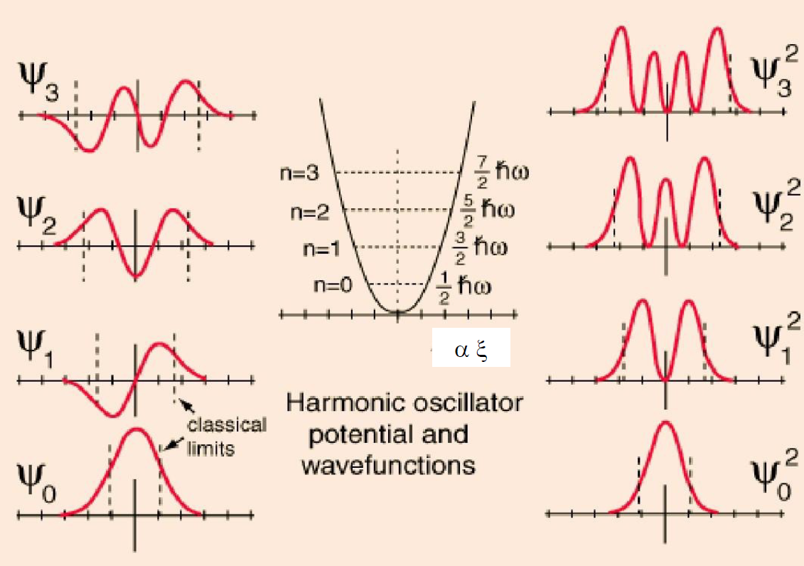
This phenomenon is called tunnelling.

6.6 Average of Potential Energy

For any state ,

We can represent with raising and lowering operators:

By orthonormality,

So

Hence we can get the kinetic

Example:

An electron confined in a harmonic oscillator ground state. The standard deviation . What is the energy needed to reach the first excited state?

At ground state, wave function is

Introduce eigenlength , the wave function is simplified:

This is a Gaussian distribution with average number 0 and standard deviation . Hence

Then

6.7 Coherent States

We first try to find the eigenstate of lowering operator.

Note that lowering operator is not Hermitian, must not be real. With a set of orthonormal eigenstates ,
according to the completeness of Hilbert space,

To simplify calculation, we need to reduce to (becuase is related with Hermitian polynomial, which is hard to calculate). To reach this target, use raising and lowering operator

Plug the coefficient into the decomposition

where is a normalization factor. Since is a constant for specific , it can be absorbed into the normalization factor.


At a later time, with time evolution oprtation,

Define ,
then

This is the eigenstate of lowering operator, called coherent state. In this state,

Since is time-dependent, the initial value is

where is the initial global phase. Plug this in,

This result indicates the average of position oscillates with time evolution, which is similar to the classical oscillator.

The standard deviation

This is a Gaussian wave packet.

7. Free Particles

7.1 Decomnposition to Momentum Space

Free particle is defined as a particle with no potential, . Its Schrödinger equation is

The general solution is

Apply time evolution,

If is allowed to take negative value, the wave function can be combined into one term

This is the standard form of planar wave. By comparing both forms, we naturally introduce dispersion relation:

According to wave mechanics, the planar wave has phase velocity and group velocity:

The definition of phase velocity is the velocity of equal-phase plane. The plane satisfies

And the group velocity is the velocity of the entire wave packet superposed by many components.

If has peak at (This means the most critical frequency component is ), expand it with Taylor series:

Plug it in,

The wave can be decomposed into two terms: carrier moves with phase velocity, and the integral term is only the function of . Hence, this term moves with velocity of . This velocity is the speed of envelope, defined as group speed.

Let’s go back to the free particle wave function.

We try to normalize it:

The wave function cannot be normalized! So, for a free particle with a definite momentum , it cannot be used as a wave function.
Or in other words, free particle has no definite energy or momentum, and it does not evolve as a planar wave. Meanwhile, the momentum in a function wave with precise is definitely determined. According to the uncertainty principle, the position of this state must be completely undetermined.

To deal with such an annoying wave function, we should use the property of . The wave function of is planar waves:

Obviously is Hermitian, the states of must be orthogonal.

So for a planar wave, we no longer require , instead, we expand the wave function into combinations of states with different momentum

and require the total normalization

where is a normalization factor. This is a Fourier inverse transformation, meaning the wave function of a free particle is a superposition of components with every values. is the wave function in the space, obtained by Fourier transdormation:

And this determines the compoents of different frequencies (imagine the frequency domain in signal processing).

Also, note that there is no quantum number in the wave function. Energy of free particles is not quantized, since there is no boundary conditions (standing wave).

7.2 Propagation of Free Particle

Since the wave function is

By Fourier transformation,

plug in to get the wave function

where

The wave function is in the form of Gaussian wave packet, which can be normalized now:

If we define velocity , parameter , then

Obviously, with time evolves, the uncertainty of gradually increases, which means the position gradually spread to the entire space. Meanwhile, according to the Heisenberg’s principle of uncertainty, the uncertainty of momentum must gradually decrease.
With time going, momentum will gather to one value and you can measure momentum more precisely.

8. δ Potential

8.1 Bounded State and Scattering State

• Bounded State: a state trapped in a potential.
• Scattering State: a state that can spread to infinite far.

Note: due to the tunnelling effect, even if a state with energy is trapped in a potential well of , there is still non-zero probability that the particle appears outside the potential well. Such states are also called scattering state.

8.2 δ-Well

Consider a potential well:

The Schrödinger equation

• Bounded State:

At , the Schrödinger equation is treated as :

Considering the boundary condition of as , the solution is:

The -function works as a boundary condition at .

Continuity at .

By normalization:

Giving .

The integration around ():

where
$$\Delta \left( \dfrac{d\psi}{dx} \right) \equiv \left. \dfrac{d\psi}{dx} \right|{+\epsilon} - \left. \dfrac{d\psi}{dx} \right|{-\epsilon}$$

Ignoring first-order infinitesimal:

Plug in the wave function

For :

Giving:

then the wave function is completely determined:

• Scattering state:

The S.E.:

Suppose the solution is:

At :

Around :

Summarize the equations:

Define

Suppose the wave is injected from left, then the 4 terms can be explained.

• A: incident wave
• B: reflected wave
• C: transmitted wave
• D: incident wave from the right. .

Delta Well and Waves

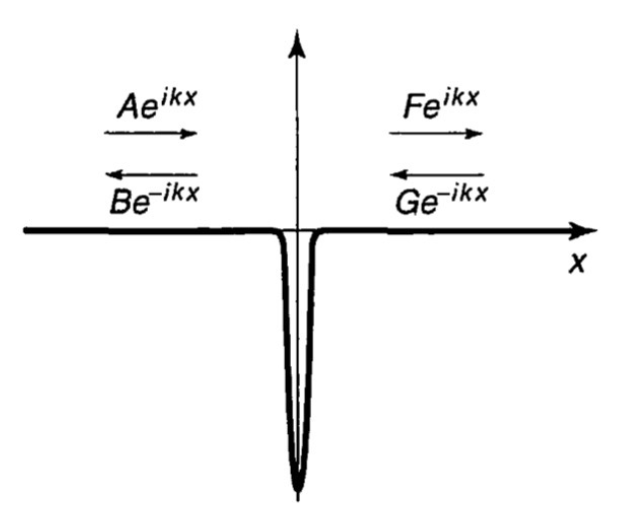
Solve the equations above.

The probability density occupied is respectively:

Define reflection rate

and transmission rate

Obviously

Indicating energy conservation.

By the way, given that ,

When increases, raises and decays. When , , which marks the intuition of classical mechanics. And for reflection, we know a sudden change of the medium will reflect part of the wave. In quantum, that’s the same.

8.3 δ-Barrier

Compared with -well, just change to . In this situation there’s no bounded states. For scattering states,

is not 0. Meaning a particle with finite energy can pass through a infinite high potential (tunneling).

9. Finite Square Potential

9.1 Finite Square Barrier

Finite Square Barrier

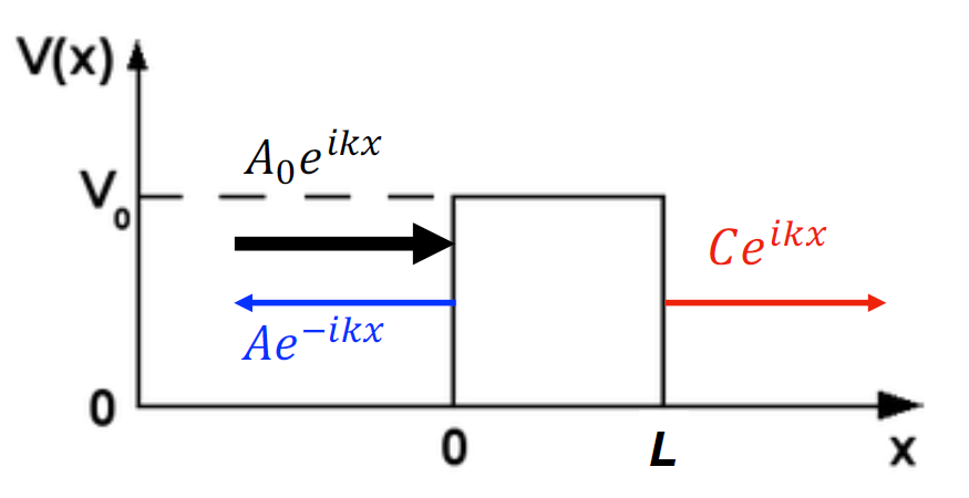
The space can be divided into 3 regions.

• ,
• ,
• , ( term vanishes because there’s no reflection wave here)

where , .

At :

At :

If use as a baseline, all waves can be expressed with .

Reflection:

On barrier:

Transmission:

The reflection and transmission rate should be

We can directly obtain

which indicates probability conservation.

In most cases in practice, , and approximately,

9.2 WKB Approximation.

For continuous potential, it can be divided into many small square barriers with infinitesimal width.

Finite Square Barrier

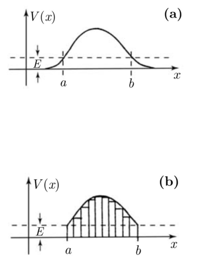
And in this case, variation of V is small. The exponential term plays much more important role than the coefficient. Hence the coefficient is regarded as 1. Then the total transmission rate should be:

This process is called WKB approximation. An application of this is -Decay. We will calculate the lifetime of radioactive isotope .

decays with the following -decay.

The radius of is

And potential of surface

In -decay, Coulomb’s force plays the major role, hence at ,

Since , the potential between and is the barrier, where .

The -decay occurs only when -particle crosses the barrier.

The transmission rate

where

Since , , approximate arcs with

This deduces

Assume -particle moves with velocity of like a free particle.

The frequency to collide the wall is:

Only of them can pass through the wall.

is the decay constant. Plug into the decay equation

Solving that

and average lifetime

Plug in data:

This is a semi-classical estimation. Compared to the experimental measurement , this result can be accepted.

9.3 Finite Square Well.

Finite Square Well

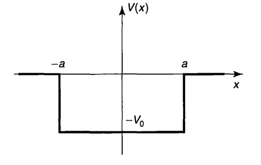
Suppose . The same method to deal with the wave functions.

where ,

To simplify, we introduce a theorem.

Theorem: If , then can always be taken to be either even or odd.

Proof. Take spatial inversion for Schrödinger’s equation:

The operators on both sides do not change after spatial inversion. Hence is also a solution. We can define two new functions:

According to superposition principle, they are also solutions of the Schrödinger equation, and are even and odd functions separately. Moreover, wave function satisfying is called state with even parity; is called odd parity.

Back to the finite square well. We suppose the square well is located between and . Then for even parity solution

with boundary condition at .

Giving

Define

gives

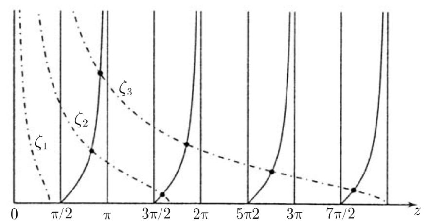
Solve the equation with figures

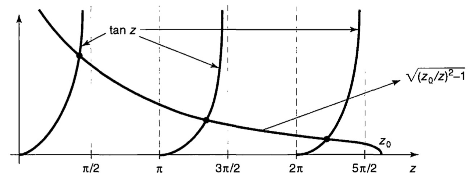
No matter how shallow the well is, there must be at least one cross point which means the bound state. In fact, the position of determines the number of bound states.

Similarly for odd parity,

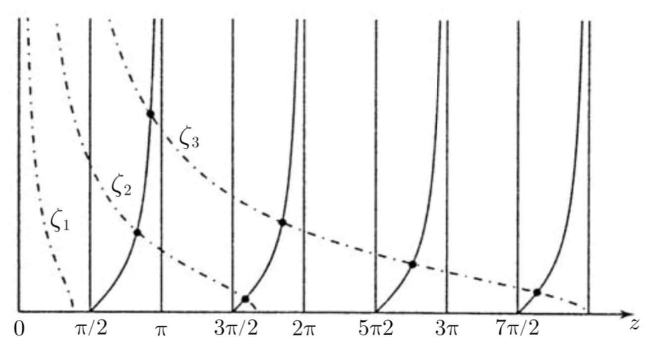
The number is

For

where ,

Apply boundary condition

Transmission rate

Note when , . The well can be regarded as transparent.

And when , , then , . The result becomes classical.

10. 3D Quantum Mechanics

10.1 3D Schrödinger Equation

Back to original Schrödinger Equation. In Central Potential

Where

Consider central potential . Define angular momentum

Mostly we discuss , representing the magnitude of angular momentum

Regardless of time, we have

By separation in variables

The two parts are independent. We define

To better apply mathematical conclusions. Recall . The equation on angles is

This equation tries to find eigenfunctions of , and is an index of rotation. To simplify notation, normalization is required separately

Further separate by

is solved by

This function is required to be periodic


Hence

is quantized.

Back to . Mathematicians say the solution is associated with Legendre polynomial.

For any given , there’re possible values of . are called orbital angular quantum number and orbital magnetic quantum number, respectively. The total solution of is given:

Normalize to determine coefficient

Plug in some values, we get some distributions.

Values of Some Spherical Harmonics

Electron Orbits of Some Harmonic Values

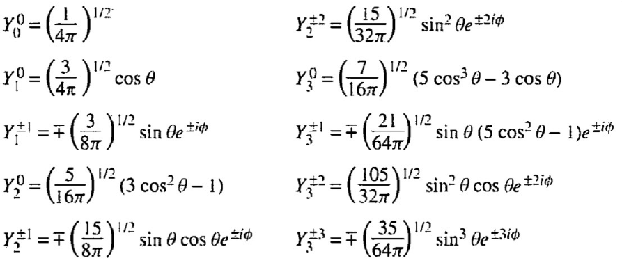
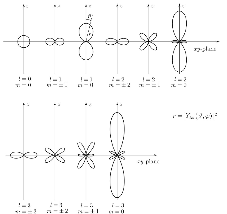
If the is in an atom, we get the orbits.

Radial equation is related to .

To simplify, define , then


The equation becomes

The new term , is defined as effective potential . The term represents the centrifugal term. For such a potential means there’s force

driving particles in it away from the center. This extra potential is introduced by angular momentum.

10.2 Infinite Spherical Potential Well

Given potential , the radial equation is given by

The most trivial case is . Then

With finite, then

The value of is determined by boundary condition

Deducing energy level

That is the energy level without rotation ().

And by normalization

It seems the result is the same as that in one-dimensional case. But the total wave function should take the angular factors into consideration

If is not zero, the general solution of the radial equation

is a combination of two types of spherical Bessel functions

Again, value of is required to be finite. Therefore

Denote th zero points of as . Then the energy level

The total wave function is

Note that is independent of in wave function, suggesting that there is a degeneracy. For the same there are valid values of . Hence, there are different states with the same energy .

10.3 Hydrogen Atom

A hydrogen atom consists of a heavy, motionless proton and a much lighter electron. The atom is mainly maintained by Coulomb potential

This is a two-body system. Such a system is equivalent to an ideal motionless center and an electron with effective mass

The mass is very close to , so we estimate with to simplify. Now write out radial Schrödinger equation

Total effective potential can be drawn.

Effective Potential of Hydrogen Atom

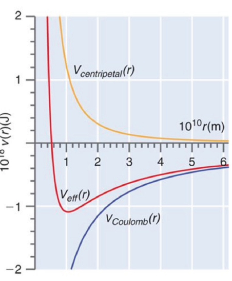
Obviously, states with are bounded while are scattered. Define

Rewrite the equation:

• Case 1,

  Approximate the equation as

• Case 2,

Approximate the equation as

giving

In general, we expect

and should have a simpler form.

Plugging into the original function, we have

To solve this equation, apply the series method. Suppose

and find a recursion equation:

is determined by the normalization condition. is defined as an associated Laguerre polynomial. If the series does not terminate (when ):

However, when , diverges, which is unacceptable for a wave function. Hence, the series must terminate at a maximum value , given by the condition :


Since is a non-negative integer, must be an even integer. To match experimental results, the principal quantum number is defined as

By the original equation, the energy is quantized:

The associated Laguerre polynomial solution is:

is the energy of the ground state.

Up till now, the total wave function of the Hydrogen atom is clear.

The ground state is characterized by:

Its energy:

To simplify the representation, define the fine-structure constant :

The ground state energy is:

This is the binding energy of the hydrogen atom. The ground state wave function is:

where is the Bohr radius:

For other quantum number combinations, the wave function is expressed with the associated Laguerre polynomial:

The normalized radial part is:

By checking the associated Laguerre polynomial , we find that it has zero points. Hence, vanishes at values of where .

Also, introduces vanishing points of . combining these results, we can draw figures of electron orbits of hydrogen atoms.

For a principal quantum number , the degeneracy of the energy level (caused by and ) is:

10.4 Angular Momentum

Recall angular momentum.

An amazing result is that any two components of do not commute.

(Calculation omitted, resulting in)

This means they have no common eigenbasis. In experiments, we can only measure one component of precisely, with the other two undetermined. However, components can be measured simultaneously with .

Also, recall is related to the angular quantum number . Analogy to harmonic oscillator operators for energy, angular momentum can be operated by ladder operators.

The commutation relation is obvious:

Given an eigenstate of and :

Applying to the eigenstate:

Applying to the eigenstate:

Obviously , so . There exists a top rung and a bottom rung.

We check the operator:

Then can be expressed as: Operate on the top rung :

Giving an equation for :

Similarly, for the bottom rung:

We know . The value of can only vary with a fixed step of , within the range of to . For states between the top and bottom rung, suppose they have a quantum number , meaning: For itself:

The normalization factor squared is:

has values of . Therefore, is an operator to raise or reduce the angular momentum on the z-direction. This result matches the solution in 11.1.

Remark. We know (except for ). This means that cannot point exactly along the -axis. Undetermined and components exist forever.

10.5 Spin

Except for orbital motion, self-rotation also introduces extra angular momentum. However, classical rotation of electrons is unacceptable, as the speed of the equator would exceed the speed of light . But experiments did detect the extra effect. We can only consider that the extra effect is a natural property, like the charge on the electrons.

Analogous to the orbital angular momentum , we introduce spin . It satisfies:

And the eigenvalue equations are:

What differs from is that is not limited by the spatial wave function, so can take half-integer values.

This result is proven by the Stern-Gerlach experiment. A beam of silver atoms is divided into 2 beams after passing through a non-uniform magnetic field. If is an integer it should be divided into 3 beams.

Ladder operators have a similar form:

The operation of the ladder operator is: The normalization factor squared is:

Remark. We have found 4 quantum numbers now:

• Principle:
• Angular:
• Magnetic:
• Spin:

Except for , the other 3 numbers , , are independent of the specific potential, so they are well-defined for all particles. depends on ; in different systems, definitions of are different. Different particles have different values, which is specific and immutable, just like electrons carrying a charge of (no one can explain why). Particles with half-integer spin are called Fermions, while those with integer spin are called Bosons.

Spin systems are the most important Fermion systems. Electrons, protons, neutrons, quarks, and leptons are confirmed to be Fermions and have spin . Such particles have two eigenstates of spin (for values):

They span a 2-dimensional space. To simplify, we can define the two vectors (spinors):

And all states can be defined as:

The spin operator:

And another important operator, .

Ladder operators are also determined by: For : The matrix results are: By the definition and , and can also be found: The total spin can be regarded as a combination of 3 components: where is called the Pauli matrix, defined as: Now comes to an arbitrary state: If operates on it:

It will definitely get the state. Sometimes we need to measure .

To find eigenvalues of :

The corresponding eigenstates are:

Any state:

can be decomposed with :

Example: Larmor Precession.

From electrodynamics, a charged particle creates a magnetic moment :

With the effect of spin:

is called the Landé factor, also a natural property of spin. If the particle is placed in a magnetic field along , the Hamiltonian, i.e., the energy, is:

Regardless of orbital motion, becomes:

where .

The eigenstates are the same as :

The eigenvalues are:

An arbitrary state with time evolution ( at ):

The mean value of should be:

It is independent of time, meaning that remains constant over time evolution, while:

This result indicates the particle precesses around the -axis. Such precession is called Larmor Precession. The frequency is obviously:

Example: Magnetic Resonance.

Any Fermions with spin of resonate with an external magnetic field. In a magnetic field along the -axis, , particles have a resonance frequency:

Now apply perturbation along the angular direction on the Hamiltonian. Let the external magnetic field oscillate with frequency :

The Hamiltonian is :

where .

The time-dependent Schrödinger Equation (S.E.) is:

The state oscillates with:

where is the detuning, and is the generalized Rabi frequency.

The solution for an arbitrary initial state is:

The most simple case is (i.e., ). With this initial condition, the probability of transition to is:

At a certain time, reaches a maximum when the external field varies with the same frequency as the Larmor frequency , i.e., . This is the resonance condition.

10.6 Addition of Angular Momentum

In quantum mechanics, angular momentum can be added. Suppose two angular momenta and commute with each other. The total angular momentum is: The -component is additive: The square of the total angular momentum is: In practice, the addition is operated by quantum numbers. The joint state is denoted by: The corresponding eigenvalue equations are: We construct the eigenbasis represented by the total quantum numbers and . This is the common eigenbasis of , , , and . The two states are corresponded by the Clebsch-Gordan coefficients: The two representations should be equal. Then: have maxima of respectively, then: For total . Now we have found the top rung of : The ladder operator under this representation is: Apply on multiple times, we construct a series of states: . At , there're states. The corresponds to the case that parallels to . Similarly, when inversely parallels to , . Meanwhile, the ladder operators ensure that can only change with interval of . Hence, for total angular momentum : For example. , then: The system has uncoupled eigenstates. For : For : We check on : For : We check on : With the basis vectors , can be expanded as a matrix: Its eigenvalues and eigenvectors are: For (singlet state): For (triplet states): Remark. is the eigenstate of . is the eigenstate of . In the example above: The uncoupled basis (eigenstates of ): The coupled basis (eigenstates of ): In the Hydrogen atom, total angular momentum . Since , we have: Magnetic dipole from : The interaction energy is . Orbital motion provides a magnetic field of (the deduction needs relativity theory). Then the potential is the spin-orbit coupling term : The total Hamiltonian is: With the effect of , and , but . Hence, are well-defined quantum numbers instead of . Obviously: Further, using , we get: The expectation value is: The expectation value of the spin-orbit potential is: where is calculated by: where is the Bohr radius. Then: Remark. It seems there's a conflict that is not well defined while it still appears in the final result. However, is a fixed number, . The "not well-defined" means that does not conserve.

In fact, if the interaction between and is ignored, are still well-defined.

10.7 Electromagnetic Interaction

Taking EMF into consideration, the Lagrangian is:

The generalized momentum is:

Hamiltonian is deduced from Legendre transformation:

According to the Ehrenfest theorem:

We calculate the commutator:

Substituting back: This leads to the classical velocity relation in quantum mechanics: The Hamiltonian can be written as:

The force in EMF is given by:

Calculate some terms first:

Recall the definition of the electric field . The terms combine to .

Now for the commutator with the kinetic energy term, we use : Next, we need :

This gives the kinetic term contribution:

Plugging in all these results, the final Ehrenfest equation for the momentum is:

If and are uniform:

That is the Lorentz force in quantum mechanics.

Quantum mechanics also introduces the Aharonov-Bohm effect, meaning that will also influence the behavior of particles, while only applies force on particles in classical mechanics.

Given an infinite-length solenoid with radius . An electron is confined on a circle with radius , whose center coincides with that of the solenoid. The solenoid carries a steady current, producing magnetic field inside, while outside remains . outside is not zero, though.

Outside the solenoid (), . In cylindrical coordinates, the component of is:

Since is independent of and , this simplifies to:

Inside the solenoid (), . Assuming (uniform):

must be continuous at :

Hamiltonian outside the solenoid () is:

The time-independent Schrödinger Equation (S.E.) for is:

Solve S.E., note that the wave function must satisfy the periodic boundary condition:

The energy level is quantumized:

The energy level depends on the flux inside the solenoid. This is a completely quantum effect, proving the physical existence of .

10.8 Hydrogen-Like Atoms

An electron is confined by a nucleus with charge , such atom is called Hydrogen-Like.

When , it is just Hydrogen atom, we have

If ,
the potential becomes times larger (absolute value) than Hydrogen. These parameters will become

When increases, -decay occurs

A neutron decays to a proton, an electron, and an anti-neutrino.

After -decay, the nucleus charge increases by 1 due to the proton produced. For an electron in 1s orbit initially, we can write the wave functions.

Before decay,

After decay,

Probability of remaining in :

For large , . Obviuosly, the larger nucleus charge is, the more probable that the electron remains on 1s.

Another type of Hydrogen-Like atom is Muonic Hydrogen (After modifying the nucleus, modify the electron). Muon is almost the same as electron, except that its mass is about 200 times larger than electron.

Back to the original equation, the ground energy becomes

Bohr radius

A system consisting of an electron and its anti-particle, a positron, bound together into an exotic atom. For double body systems,
we will introduce reduced mass

This system is equivalent to a particle with mass rotating around an ideal central potential field.
With hydrogen energy level

Replace with

10.9 Infinite Square Well

An electron is confined in a 3-D box, calculate the ground state energy and 1st excited state energy.

3D Infinite Square Well

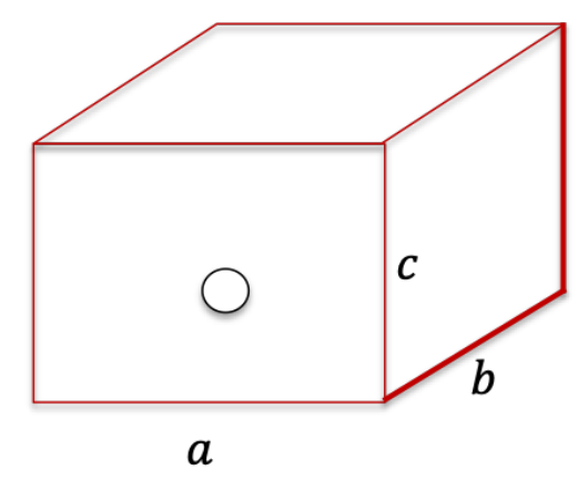
The 3D TISE gives

Under Descarte coordinate

This equation can be solved by separation of variables:

And

Boundary condition indicates

Solving the wave function

Total wave function

The solution is similar to 1D infinite square wall. The energy level

The ground state should be .

10.10 Finite 3D Spherical Potential Well

Radial TISE gives

when (ground), at ,

Solving,

Boundary condition yields , then .

At ,

Solving,

Boundary , yielding hence

Continuity yields

According to the figure below, bound states exist only when

yielding

11. Identical Particles

11.1 Bosons and Fermions

Fundamental particles are ususally undistinguishable. You cannot say if the electron in a hydrogen atom is replaced by another electron, it is no longer a hydrogen atom.

Let’s consider a two particle system,

Define exchange operator.

Obviously,

Its eigenvalues are therefore . The two eigenvalues correspond to two types of particles. If

Such particles are called Bosons.

If

Such particles are called Fermions.

To decouple the wave function of the two particles while display the symmetry explicitly, we usually reassign the joint wave function:

This form is equal to the original separation . The energy is still

Due to the anti-symmetry, Fermions have an exotic property. Consider a Helium atom, with two electrons on 1s. The wave function is

Let , the amazing result will be

meaning the probability of finding two Fermions with the same place is exactly 0. This is the Pauli exclusion principle.

Experiments found that Bosons have integer spin and Fermions have half-integer spin.

11.2 Two Particle Systems

Symmetry of wave function introduces force, which can be made clear by inspecting .

For distinguishable particles

Then

For identical particles, the wave function should be equivalent to

Then these terms are

where

Then identical condition yields an extra term

The extra term indicates that Bosons tend to be closer and Fermions farther apart.
The term exists only when and actually overlap. Macroscopically, the new term behaves as a force.

Experiments found that there’s 2 electrons in orbit of Helium, which seems to violate the Pauli Exclusion Principle. To solve the problem we introduce spin. The total wave function of an electron is

The joint wave function is

The joint wave function must be anti-symmetric, i.e., one of the wave functions, spatial or spin, is symmetric and another is anti-symmetric. No one cares which one is symmetric on earth.

Take an example of Helium (). Its Hamiltonian We ignore the less important but most troublesome interaction term, then the equation separates. Then the total spatial wave function is simply the product of two hydrogen results. with half the Bohr radius and times Bohr energy. The total energy The ground state is Helium total wave function are also compared by

We have configurations to satisfy anti-symmetry. If is anti-symmetric, this configuration is called parahelium (singlet), otherwise , , called orthohelium (triplet).

For atoms with more electrons, since electrons are identical Fermions, subject to Pauli’s exclusion principle. Only two electrons can occupy one orbital position due to the variation of spin. Similarly for other quantum numbers . Finally, one position of fix is called a shell and a shell can carry at most electrons.

Now let’s consider only the outermost electrons. Since the inner (layers’) total orbital and spin angular momentum and are only composed by the outermost layer. Moreover, the total angular momentum can take values

The total quantum numbers config an atom with fixed

Energy of these configurations are predicted by Hund’s rule:

• States with the highest total spin will have the lowest energy.
• For a given spin, states with the highest total orbital angular momentum will have the lowest energy.
• If is no more than half filled, the lowest energy level has , otherwise has the lowest energy.

11.3 Free Electron Gas

Solid, especially metal, is composed by (almost) fixed positive nucleus and uniform electron gas. Other examples are also common, like neutron star, composed by free neutron gas, another Fermion gas.
Suppose the object is a rectangular solid, with dimensions . The electron gas experiences potential

The S.E. can be solved by separation of variables.

Apply boundary condition

Similarly


Total

And the allowed energy are

where

Let’s turn to the space. From the solution above, an electron occupies one integer coordinate . Suppose there’s electrons (usually large on the order of ). By the property of Fermions, only electrons can occupy the same . Since particles tend to occupy states with lower energy first, large number of electrons fill up an octant of -sphere, whose radius is determined by the fact that each pair of electrons require a volume . (Each point in space occupies volume because are discrete points. This is an average equivalence.)

Thus

where is the number density of electrons. The sphere surface is called Fermi surface, called Fermi radius. The threshold energy, determined by

is called Fermi energy.

The total energy of the entire Fermion gas is

This total energy is analogous to the internal thermal energy, and it shows up as a pressure on the wall.

This pressure is mainly caused by Pauli’s exclusion principle, called degeneracy pressure. Someone may be confused by the disappearance of Coulomb force. We ignore them because they are approximately shielded by the fixed nucleus. Under large , these nucleus can be regarded as a uniform, positive background. This background shields negative charge very well.

11.4 Band Structure

Now improve the electron gas (not all Fermions) by including the positive nuclei. With these nuclei, the potential is no longer 0 inside the solid, but becomes a Dirac comb.

   

  Periodic Delta Potential in Solid

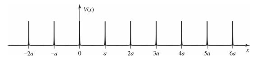
For such periodic potential , Bloch’s theorem tells that the solution to S.E.

satisfies

where is some constant independent of . It means

For solid containing very large number of nuclei and electrons , boundary where periodicity is spoiled cannot affect the property significantly. This suggests that forcing the correction of Bloch’s theorem

will not cause too much effect under on the order of . It follows by

Finally the constant is given by

Now the solid are completely periodic. With the potential

we can solve only one cell and apply to find the total wave function.

In the region .

The general solution is

The wave function in the left cell


At , the continuity of wave function yields

Discontinuity of derivative yields

The two equations are simplified to

Define , , then the RHS

Notice that oscillate outside range , so for satisfying , there must be no solution. These regions are called forbidden gap. The energies are called forbidden energies. Allowed regions, which , are called bands. Within a given band all energies are allowed due to where is very huge.

   

  Periodic Delta Potential in Solid

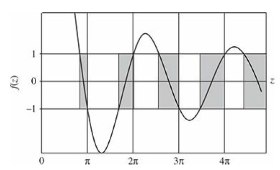
The results above are about one electron. If atoms are in the potential, each with electrons, only two of them can occupy one band, since the band structure is global. Since and is a huge number, each corresponds to a unique value , determining an energy level. Since is even, while is defined on , so the first band region for is not , but

This region is called the first band. We can similarly define other bands. Each is an energy level, so one band contains at most electrons.

If , first band will be half-filled , if completely filled ; , second band half-filled … So, if the topmost band is only partly filled , it takes a very little energy to excite an electron to the next level. Macro-copically, it behaves as conductor. On the other hand if the topmost band is completely filled, it costs too much energy to overcome the forbidden gap, behaving as insulators. If the gap is rather narrow, exciting is not as easy as conductors but also not as difficult as insulators, such materials are called semi-conductors.

In the free electron gas, all solids should be metals.

12. Symmetries and Conservations

Symmetry means that some transformation leaves the system unchanged. For example a rectangular remains unchanged after rotation by 90 degrees. We say it has discrete rotation symmetry. Obviously a circle has continuous rotation symmetry.

Before proceeding, we need to define some operators on space.

Translation operator

This operator shifts the wave function a distance to the right.

Parity operator

This operator changes the sign of these three coordinates.

Rotation operator

This operator rotates the wave function counterclock along the axis.

12.1 Transformation in Space

A translation operator can be expanded:

Hence

We say is a generator of .

Obviously inverse of is itself because translation is invertible, and

Thus is unitary.

The translation of operators is defined to be the operator that gives the same expectation value in untranslated as the original operator in the translated

To understand this, we can say moving the wave function (system) right is equivalent to moving the operator (measuring point) left. It may be confusing why corresponds to moving left. Let’s inspect this operator, suppose

Now it is clearer.

An example is momentum . Since

It remains unchanged because momentum is independent of where the original point is, depending only on the differences. This property is called translational invariance.

Now we know behavior of any operators under translation

For example, Hamiltonian

Its translation is

If , we know

The potential should be periodic (discrete translational symmetry) or constant (continuous translational symmetry).

In periodic potential, we have introduced Bloch’s theorem. We re-prove it, more precisely.

where since is unitary. We can say . We just write for some practical reasons on solid physics. Then

More illuminatingly, we write it in a new form

where . is a travelling wave. You can derive one form from another form.

In constant potential, it’s useful to consider an infinitesimal translation.

Continuous translation tells commutation.

According to Ehrenfest’s theorem.

yielding momentum conservation.

12.2 Conservation Law

Conservation in QM means the expectation and the probability of getting any eigenvalue is independent of time, for an operator . Also, according to Ehrenfest’s theorem

The operator does not explicitly depend on time. Then if ; On the other hand, probability of getting must be a constant. If the two are both satisfied, we can say conserves.

We prove it precisely now. Since and commutes, they have common eigen-basis. Let.

where . The probability of measuring is

which is clearly independent of time.

12.3 Parity

In one-dimension cases parity operator implements inversion.

Evidently

And

Thus

Its eigenstates are even or odd, with eigenvalue or , respectively.

Operators transform under spatial inversion is

Position and momentum are both odd

Then any operator transforms

If

then we say has inversion symmetry. This indicates

According to Ehrenfest’s theorem, if has inversion symmetry,

If is a Hamiltonian, it means parity is conserved if a particle moves in a symmetric potential. An odd wave function remains odd at any time and so does even.

In 3D spaces,

Evidently, in a central potential

because

Parity selection rules tell when a matrix element is zero based on the symmetry. We illustrate it with an example of dipole

The parity,

It is therefore odd. Now consider the matrix elements between two eigenstates in a central potential.

We see immediately that

This is called Laporte’s rule, saying the matrix element vanishes between eigenstates with the same parity.

This rule can be applied to any odd operator.

If is even, i.e. , then

The element vanishes when is odd.

Vectors and scalars are classified as true or pseudo- based on their commutation relations with parity .

• , is a true vector. It is odd under parity transform.
• , is a pseudo vector. It is even under parity transform. Tangent component remains constant before and after mirroring.
• , is a true scalar.
• , is a pseudo scalar.

12.4 Rotational Symmetry

The rotation operator

Similarly to the translational operator,

Giving

The same, is the generator of rotations about axis.

Obviously, position vectors are transformed by rotation operator can be considered as a matrix product.

In 3D cases, rotations are related to directions.

where is the normal vector in that direction. This operator rotates the wave function along direction .

Rotation is a vector operator. Any vector is transformed in the same way with

Back to the matrix above. If we take an infinitesimal rotation.

Apply to the vector

Write it in a more compact form by comparing with reduced infinitesimal matrix

We get

For a particle of mass moving in a potential , Hamiltonian

is rotationally invariant if is central (). In this case

For infinitesimal rotation

which means

By Ehrenfest theorem

Thus, continuous symmetry leads to angular momentum conservation. shows also commutes with . , and form a complete set of compatible observables for the bound states of a central potential. Such a set of observables has common orthonormal eigenbasis and can determine the state of a quantum system uniquely, with no degeneracy.

---

Like parity, rotation has its own selection rule. This rule is also called Wigner-Eckart theorem.
For scalar operators, commutation of scalar operator with angular momentum can be written in

Then operator satisfies retation invariance. Now take state which

Take matrix element

Hence,

The raising and falling operator can give more information.

When and , the coefficients are equal and cancelled. Then

To summarize,

the term is called reduced matrix element. For scalar matrix, it is just diagonal elements, this coefficient indicates the physical information.

---

We then move to vectors. We begin by defining raising and lowering operators.

We get commuting relations.

We apply the same operation to find matrix elements.

We can summarize

If necessary the expression can be transformed into and

The remaining commutations introduce Clebsch-Gordan coefficients.

To summarize, when , , the first gives

The second, with application of ,

Giving The third

In general, with , we have a recursion relation.

Clebsch-Gordan coefficient follows the same recursion. Thus, we can introduce CG coefficient.

where

The essence why CG coefficient appears here is that operators also carries angular momentum. A scalar operator has and are unchanged by rotation. A vector operator has , acting the same as angular momentum. The two relations between matrix elements and their reduced elements are called Wigner-Eckart theorem.

12.5 Degeneracy

Symmetry leads to degeneracy. A symmetry implies

If we have a stationary state , then is a stationary state with the same energy. The proof is trivial.

Not all symmetry leads to degeneracy because the two states and might be the same. If , the operation does not generate new state, then no degeneracy occurs. In fact only a single symmetry operator does not introduce degeneracy because we can always find simultaneous eigenstates of and and these states are transformed to themselves by . If there are multiple commuting operators, it is the same case.

Degeneracy often occurs when there’re two non-commuting operators but they both commute to . First consider a state .

Since , then

Since , there cannot exist a complete set of simultaneous eigenstates of all three operators . Then, there must be some states that is distinct from , generating new physical states. But commutation of and guarantees that and shares the same energy. Thus, the presence of multiple non-commuting operators guarantees degeneracy of energy spectrum.

12.6 Translation in Time

In sections before, we have derived time evolution operator from time-depended S.E.

Like other operators, time evolution on an operator is

The transformed operator is called Heisenberg-picture. For example, Hamiltonian is written as

An infinitesimal time translation

Apply Heisenberg-picture, the position is

We have been working on Schrödinger picture for a long time, which time translation is applied on state

But this is evidently equivalent to Heisenberg picture

If the time translation operator is independent of the time origin point, i.e.,

for any arbitrary choice of , then we say the system has time-translation invariance. This means if the system is in at both and , then it will transform to after the same time interval. This also means

Evidently

Accordingly to Ehrenfest theorem

Therefore, energy conservation is a consequence of time-translation invariance.

13. Perturbation Theory

13.1 Nondegenerate Perturbation Theory

Suppose we have solved S.E. for some exactly given potential.

obtaining a complete set of orthonormal eigenbasis

Now the potential is slightly perturbed, generating new set of eigenbasis.

In most cases we cannot solve the new S.E. exactly. The perturbation theory is applied. We write the new Hamiltonian into 2 terms.

where superscript of means unperturbed. is the perturbation. The wave function and energy are both corrected, by expanding by .

The small perturbation introduces infinite orders of correction. To simplify, absorb the factorials.

Here are the order correction. Plugging in .

Collecting like power of

Correspond coefficients of different orders, we get

The parameter is in fact a mathematical trick. It just keeps track of different orders. After all analysis, we just let and it converges to the physical system.

---

We now focus on the first order

Take inner product with

Since is Hermitian

Then

We can say the first order correction to energy is the expectation of the perturbation in the unperturbed state. For wave function:

Rewrite it

Since unperturbed wave functions form a complete set of basis, can be decomposed by

The reason why is not included is that we expect normalization even after perturbation, i.e.

To satisfy normalization, we require

This requires the linear combination should not include term. Plug in

Take inner product with

If , we recover .

If :

Then

So

The denominator is safe if the energy spectrum is nondegenerate.

---

Proceeding as before, the second order:

Again

Then

But , then

The method to get is the same.

13.2 Degenerate Perturbation Theory

If degeneracy exists in the system — and share the same energy, then the ordinary perturbation fails. Suppose

Then any combination

satisfies

Typically perturbation spoils degeneracy. splits into two as increases from to . When we turn off () perturbation, the splitted states go back to degeneracy. The upper state collapses to a combination of and and the lower state collapses to another orthogonal state. But before calculation we do not know the combination exactly. In fact the collapsed states are defined as

We call it “good states”. Now we solve S.E.

with

Plug in

The first terms cancel.

Take inner product with

Plug in weight []

Then

Similarly for

The two equations derives linear equations:

We define

We now can say the “good states” weights are the eigenvector of matrix . The equation can be written in a compact form:

This equation is called secular equation. Solve it

The two roots correspond to the two perturbed energies. When perturbation is turned off, the states go back to its corresponding eigenvector. If we want let to be the good states, we should make the eigenvectors to be and . This happens when

Thus, if we select the “good states” as a basis of the degeneracy subspace, the perturbation Hamiltonian will be diagonal, simplifying the secular equation. Besides, under perturbation, degeneracy is spoiled, and the good states can be considered as two non-degenerate states. Then in the following steps, non-degenerate perturbation theory can be applied. However, if degeneracy is not spoiled in some special cases, we have to apply secular equation in the smaller degenerate subspace, and find a second order good states.

To determine the good states, we have a theorem.

---

Theorem: Let be a Hermitian operator. If and , and if

Then and are “good states” in perturbation.

Proof. . Since and commute, there exists simultaneous eigenstate where

We can say is all states in degenerate subspace.

Take inner product for

Thus

Similarly

Take limit as

We have . This means is in the degenerate subspace spanned by and .

In this set of states, only two are allowed:

Now we can say the are already the good states. In the proof above we only care about the states that converge to degenerate energy when perturbation is turned off ().

When higher degeneracy occurs, the matrix raises its order.

And the good states becomes

13.3 The Fine Structure of Hydrogen

The fine structure is more precise than Bohr’s model, mainly caused by relativistic correction and spin-orbit coupling. Classical Hamiltonian is given by

First we focus on relativity. In relativity, the first term of Hamiltonian (kinetic) is

In classical limit, expand it:

The lowest order of relativistic perturbation is

The first order perturbation energy is

S.E. for unperturbed states says:

Then

where is the Bohr energy, indicating unperturbed energy. Let be Bohr radius, apply to calculate expectation

Then, plug into and eliminate with

Though hydrogen atom is highly degenerate, the perturbation is spherical symmetric and therefore

And is also spherical, then

Then according to the theorem in the last section, are good states, we can apply nondegenerate perturbation theory directly. The energy correction is directly given by

---

On the other hand spin-orbit coupling introduce perturbation Hamiltonian

where the magnetic field is generated by electron.

The magnetic dipole moment is caused by spin.

Then

But Thomas precession throws an extra, non-neglectable correction. The electron accelerates and its static frame is non-interial. Thomas precession says its angular velocity is

Coulomb force provides acceleration

Plug in

The correction

Then perturbation energy is

With spin-orbit coupling, , . However, , , and also commutes with total angular momentum

Thus

For electrons

and we conclude

Noting that and are in the same order, so we can add them together to get the total correction energy. With , . When

If you let , surprisingly you’ll get the same result. Hence

The correction breaks degeneracy of . Different will perturb the energy with different correction values.

13.4 Zeeman Effect

When an atom is placed in external magnetic field, the perturbation Hamiltonian is

---

If , fine structure dominates. We treat as unperturbed and as perturbation. Unperturbed states are , and unperturbed energies are . Suppose is aligned along axis, . Then Since is a constant. On time average, is a projection of Thus The coefficient is called Landé factor The perturbed energy is thus where is called Bohr magneton. In weak external magnetic field, energy level splits, so-called Zeeman effect.

---

If , Zeeman effect dominates, and perturbation becomes , while unperturbed . The unperturbed energies are calculated with We use and here because unperturbed Hamiltonian is defined by and and no spin-orbit coupling included. We are lucky that are good states because commutes with both and because , and dominates in . In first order perturbation theory, The relativistic term are the same. For the spin-orbit term, Then This is called Paschen-Back effect.

13.5 Time Dependent Perturbation

Consider two states

and the initial state is

The final state after time

Now apply a small, time-dependent perturbation , the state should also be time-dependent

where the perturbation is absorbed in and . Suppose at , , and after some , , , then we say a transition from to occurs.

To research transition, we plug in perturbation into S.E.

Plug in , we get

Reassign it, take inner product with

Giving a differential equation Similarly for Define frequency

and new coefficients

Then

Similarly If there's no perturbation, we have and , which is the order condition. With perturbation, on the first order we should consider the effect of and .

Then

Now we insert and to the RHS of equations to obtain the second order approximation.

These equations give the second order correction.

---

References:

[1] P. A. M. Dirac, The Principles of Quantum Mechanics, 4th ed. Ely House, London: Oxford University Press, 1958.
[2] D. J. Griffith, Introduction to Quantum Mechanics, 3rd ed. Cambridge: Cambridge University Press, 2018.