Calculus

Copyright Notice:
This article is licensed under CC BY-NC-SA 4.0.
Licensing Info:
- Title: Calculus
- Author: EleCannonic
- Link: https://elecannonic.github.io/categories/math/calculus/
Commercial use of this content is strictly prohibited. For more details on licensing policy, please visit the About page.
1. Set Theory and Functions
1.1 Generalized Distributive and De Morgan’s Laws
Consider a family of sets
Distributive Law:
De Morgan’s Laws:
Proof of the Distributive Law:
Use (1) as example:
Let's prove the first equation.Proof of De Morgan’s Law:
Use (3) as example:
Let's prove the third equation.1.2 Fundamental Properties
1.2.1 Spare Rational Number
Consider the set of rational numbersLet’s take a value
1.2.2 Upper and Lower Bounds of
Since 1.2.3 Countability
Definition: A set is countable if its elements can be arranged into a sequence according to a certain rule.
Every finite set is countable, but not every infinite set is countable.
Consider1.2.4 Cartesian Product
Definition: For any element
1.2.5 Functions
A function is defined by its rule:The conditions for a function are:
Domain
Codomain
Uniqueness
Injective (One-to-one): No two values map to one.
Surjective (Onto): Every element is mapped.
Bijective (One-to-one correspondence): Both injective and surjective.
Proposition for injectivity:
Note: Each element in the domain must map to a unique image, but a unique image does not require a unique pre-image.
Boundedness: A function is bounded if there exists
Monotonicity: Strictly monotonic
Periodicity, Parity, …
2. Sequence
2.1 Continuity of Real Number
Natural numbers are defined by the following 5 axioms (Peano Axioms):
1 is a natural number.
Every natural number has a successor.
1 is not the successor of any natural number.
The successor is unique.
(Principle of Mathematical Induction) If
is a proposition about natural numbers such that
Natural numbers (closed to plus and multiply) are extended to integers (
2.1.1 Upper Bounds and Lower Bounds
Definition: Let
Upper bound: Least upper bound sup
Lower bound: Greatest lower bound inf
Properties of the least upper bound (sup): (Let
is an upper bound of . . - Any number smaller than
is not an upper bound. .
2.1.2 Supre- /Infimum Existence Theorem
Theorem: Every non-empty set of real numbers that is bounded above has a least upper bound (supremum). Every non-empty set of real numbers that is bounded below has a greatest lower bound (infimum).
Pf.For all
Here,
Let
Then any set of real numbers
…
This implies:
Let
Step 1: Prove
If
- (*) There exists
such that - (**) For all
,
If case (*) holds, then
If case (**) holds, then by comparing digit by digit, we get
Step 2: Prove that for every
For any
Take
Therefore:
That is,
Theorem: The supremum and infimum of a non-empty bounded set of real numbers are unique.
2.2 Sequence Limits and Infinitesimals
2.2.1 Definition
Let2.2.2 Properties
- Uniqueness: The limit of a convergent sequence must be unique
Pf.: Take
- Boundedness: A convergent sequence must be bounded
Pf.: Assume
Note: A bounded sequence may not necessarily converge.
- Order Preservation: If
, both converge, , , and , then ,
Pf.:
TakeDef: Sequence with limit equals to 0 is called a infinitesimal.
2.3 Arthematic Operations of Limit
2.3.1 Pre-conditions
These introduce two relations:
2.3.2 Summation
Pf.
2.3.3 Production
Pf.
2.3.4 Division
Pf.
Take2.3.5 Squeeze Theorem
IfPf.:
2.4 Infinite Sequences
2.4.1 Definition
A sequenceNote: Infinite sequence ≠ Unbounded sequence. Counterexample: 1,1,2,1,3,1,4,1,…
2.4.2
Theorem: If
Pf.
(i) If
(ii) If
2.4.3
Theorem: If
Pf.
Corollary: If
2.4.4 Arithmetic Operations of Infinite Sequences
2.4.5 Stolz Theorem
Definition: If
Stolz Theorem: Let
Pf.Case 1:
Case 2:
Case 3:
e.g. 1: If
e.g. 2:
2.5 Convergence Criteria (Real Number Continuity Theorem)
2.5.1 Monotone Convergence Theorem
A monotone bounded sequence must converge.
Pf.Assume
e.g.: Nested Radical Limit
Prove the existence of
(i) Boundedness: Prove
(ii) Monotonicity: Prove
2.5.2 Fibonacci Sequence Growth Rate
Fibonacci sequence:2.5.3 The Number
Pf.:
2.5.4 p-Series Convergence
LetCase 1:
Case 2:
2.5.5 Harmonic Series and Euler’s Constant**
Let2.5.6 Nested Interval Theorem
Definition: A sequence of closed intervals satisfying two conditions:
Nested Interval Theorem: If
Pf.By the definition of nested intervals,
e.g.: Prove
Method 1: Nested Interval Theorem
Proof by contradiction. Assume- This is a nested sequence of closed intervals
,
Method 2: Diagonal Argument
It suffices to prove2.7 Subsequence
2.7.1 Definition
SupposeTheorem: If
Pf.
Corollary: If
Theorem:
Pf.
Sufficiency is obvious.
Necessity: By contradiction, assume that
That is,
Any subsequence of
2.7.2 Bolzano-Weierstrass Theorem.
A bounded sequence must have a convergent subsequence.
Pf.
Suppose
Repeat this process to obtain a nested sequence of closed intervals
Take
Take
Take
…
We obtain a subsequence
2.7.3
Theorem. If
Take
Take
…
We obtain a subsequence
2.7.4 Theorem
If
Take
Take
…
We obtain a subsequence
2.8 Cauchy Convergence Principle
2.8.1 Cauchy Sequence
Definition (Cauchy Sequence):
e.g.:
Pf.
Take
e.g.:
Pf.
If we take
2.8.2 Cauchy Convergence Principle:
Cauchy Convergence Principle:
Pf.
- Sufficiency:
Assume
Then
For any
Hence,
- Necessity:
First, prove that any Cauchy sequence is bounded. By the definition of a Cauchy sequence,Then Let Then
By the Bolzano-Weierstrass theorem, there exists a subsequence
Also,
For any
Thus,
Contraction Condition: If
Pf. Show that
3. Functional Limit
3.1 Definition and Properties
3.1.1 Definition of functional limit**
**Definition:** Supposee.g. Prove
Pf.
3.1.2 Heine Theorem**
The necessary and sufficient condition forTheorem: The necessary and sufficient condition for the existence of
3.2 Properties of Functional Limit
- Uniqueness: If
are both limits of at , then .
- Squeeze Theorem: If
, is satisfied. And , then .
Four Arithmetic Operations: Suppose
.
- Local Sign-Preserving Property: If
and , then in a certain deleted neighborhood of , there always exists .
Corollary:
- If
, then , s.t. - If
, and , s.t. , , then . - If
, then , s.t. is bounded in .
3.3 Single-Sided Limit
**Definition:** LetTheorem.
e.g. Heaviside Function
Functional Limit Definitions can be expanded. Consider a limit
“A” can be
“B” can be
e.g.
3.4 Continuous Functions
3.4.1 Continuity
Definition. Suppose
Requirements:
- Both left and right limits exist and are equal.
- The function value exists and is equal to the limit.
(1) Continuity on an open interval.
If
e.g. Prove
Take any
Let
By definition,
(2) Continuity on a closed interval.
One-sided continuity: If
If
Continuity on a closed interval: If
e.g. Prove
Take any
then
Considering endpoints,
Hence
In summary,
If
Conclusion:
- Any polynomial
is continuous on . - Any rational function
is continuous on its domain.
3.4.2 Discontinuity
(1) Types of Discontinuity Points
Type I (Jump Discontinuity): Left and right limits exist but are not equal.
- e.g.:
, , etc. - Definition of jump magnitude:
- e.g.:
Type II: At least one of the left or right limits does not exist.
- e.g.:
,
- e.g.:
Type III (Removable Discontinuity): The limit exists, but the function value does not exist or is not equal to the limit.
- e.g.:
- e.g.:
e.g.: Thomae’s Function (Riemann Function)
(
Fact:
Pf.
For example, there will not be more points than those in the following table (taking the interval shown below):
Let the rational number satisfying condition (*) that is closest to
Let
- If
, then . - If
, the distance from to is closer than , i.e., .
By the definition of
(2) Discontinuities of Monotonic Functions
Theorem: Discontinuities of a monotonic function on
Pf. Assume
Let
Similarly,
If
Proof by contradiction: Suppose
① If
② If
In summary, the proposition is proven.
Theorem: A monotonic function has at most countably many discontinuities.
Pf. Without loss of generality, assume
Since a monotonic function can only have Type I discontinuities, for
By the density of rational numbers,
(3) Continuity of Inverse Functions
If
Theorem: Suppose
Pf. First prove
Next, prove continuity. Take any
Finally, prove
(4) Continuity of Composite Functions
Note: If
Theorem: If
Pf.
Furthermore, due to the continuity of
In summary,
Thus,
3.5 Infinite Quantities
3.5.1 Infinitesimals and Their Orders
Definition (Infinitesimal): If
Comparison: Suppose
- If
, then is a higher-order infinitesimal of as .
We denote this as. - If there exists
, s.t. in a deleted neighborhood of , , then is bounded relative to as .
We denote this as.
Theorem:
If there further exists
- If
, then and are infinitesimals of the same order. - If
, then and are equivalent infinitesimals, denoted as .
Order of Infinitesimals: If
is an infinitesimal. is bounded.
As
As
3.5.2 Comparison of Infinities
Definition (Infinity): If
Comparison: Suppose
- If
, then is a higher-order infinity of as . - If there exist
, s.t. , , then is bounded relative to . We denote this as .
Note: Higher-order infinitybounded. - If there exists
, s.t. , , then and are called infinities of the same order as . - If
, then and are equivalent infinities as , denoted as .
3.5.3 Equivalent Infinitesimals
(1) Common Equivalent Infinitesimals
Let. As , .
Let. As , .
(2) Applications of Equivalent Infinitesimals
Theorem: Suppose
Pf.
Theorem: If
Pf.
Example:
3.6 Continuous Function on Close Interval
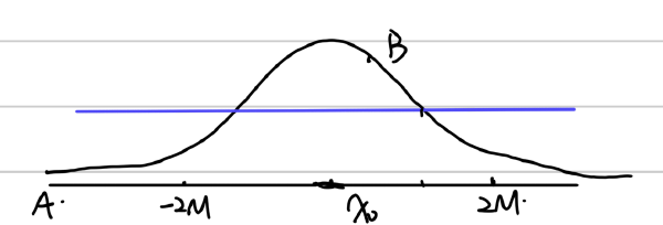
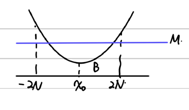
3.6.1 Boundness Theorem
If
Boundedness Theorem: If
Pf. (Using Nested Intervals Theorem): By contradiction. Suppose
Let
Bisect
Repeating this, we obtain a sequence
By the Nested Intervals Theorem,
Since
Since
This contradicts the fact that
Pf. (Using Bolzano-Weierstrass Theorem): By contradiction. Suppose
By the definition of unboundedness,
We obtain a sequence
By the Bolzano-Weierstrass Theorem,
However,
Pf. (Using Finite Covering Theorem):
By the local boundedness of continuous functions,
Let
By the Finite Covering Theorem,
Let
Then
Thus
Therefore,
3.6.2 Extreme Value Theorem
Theorem (Extreme Value Theorem): If
Pf. If
Since continuous functions on closed intervals are bounded, by the Axiom of Completeness,
Let
We obtain a bounded sequence
s.t.
We have
By the Squeeze Theorem and the continuity of
Thus
The existence of
3.6.3 Zero Point Theorem
Theorem (Zero Point Theorem): If
Pf. (Using Nested Intervals Theorem): Assume without loss of generality
If
If
If
Assume
If
If
If
If the proof does not terminate in finite steps, we obtain a sequence of nested intervals
By the Nested Intervals Theorem,
By the continuity of
Since
3.6.4 Fixed Points
(1) Fixed Point
Theorem: Suppose a continuous function
Pf.
Thus
If
If neither is 0, then
(2) Contraction Mapping Theorem
Definition (Contraction Mapping):
Contraction Mapping Theorem: If
Pf. 1:
Let
If
By the Fixed Point Theorem,
Uniqueness: Assume
Pf. 2:
By the Fixed Point Theorem,
Arbitrarily pick
For
Then we have:
Since
By the Cauchy Convergence Principle,
Since
Thus
If
3.6.5 Intermediate Value Theorem
Theorem: If
Pf.
By the Extreme Value Theorem, let
Without loss of generality, assume
Pick any
Then
Applying the Zero Point Theorem to
That is,
Corollary: If
3.6.6 Uniform Continuity
Continuity on Interval
Definition (Uniform Continuity): Suppose
Intuitive Explanation: In general continuity,
Example:
Contraction mapping is definitely uniformly continuous.
Theorem:
Note: It is not required that
Pf.
Necessity: Suppose
Since
Thus
Sufficiency: By contradiction. Suppose
Take
We obtain
Theorem (Cantor’s Theorem): If
Pf.
Suppose
By the Finite Covering Theorem,
Let
Take any
Then
Therefore
Theorem: Suppose
Pf.
Sufficiency:
Take a sequence
By the uniform continuity of
By Heine’s Theorem,
Thus
Therefore
Necessity: By contradiction. Suppose
Take any
Take
Take
We obtain a sequence
By Heine’s Theorem,
Due to the arbitrariness of
Thus
4. Differentiation
4.1 Differentiation and Derivative
4.1.1 Differentiation
Suppose
is linear: is proportional to . is non-linear but locally smooth at : When and are very small, .
Definition (Differentiability): Let
then
Basic Properties:
- If
is differentiable at , then as . - If
, then as . is called the linear principal part of .
Definition (Differential): If
Example:
Let the differential of the independent variable be
Example:
Note: Differentiable function must be continuous, but it’s not correct in the opposite direction.
4.1.2 Derivatives
If
Dividing by
Definition (Derivative): If
This limit is denoted as
Derivative Function: If
The derivative at each point defines a new function
Theorem:
Pf.
Derivable
Suppose
This implies
Thus
Therefore
3. Geometric Meaning of the Derivative
- Secant line: The slope of the secant line is
. - Tangent line: If
exists, then has a tangent line at . - Equation of the tangent line:
.
4.1.3 One-Sided Derivatives
Definition: If the limits
Theorem: The necessary and sufficient condition for
The derivation of this follows directly from the conditions for the existence of a limit.
e.g. Given
Prove that
Pf.
Since
Assume by contradiction that
Then for the right derivative:
And for the left derivative:
$\implies f’+(\dfrac{1}{2}) \ne f’-(\dfrac{1}{2})
4.2 Arithmetic Rules for Derivatives
4.2.1 Proofs of Common Derivatives
4.2.2 Arithmetic Rules for Derivatives
Theorem. Suppose
Pf.
(1)
(2)
Let:
Then
Generalizations.
(1)
(2)
Theorem. If
Pf.
Theorem. If
Pf.
4.2.3 Differentiation of Composite Functions
Theorem. Suppose
Proof. Let
Since
Since
Thus,
Formally:
Theorem (Multiple Chain Rule):
4.2.4 Differentiation of Inverse Functions
Theorem. Suppose
Proof. By the Inverse Function Continuity Theorem,
Strict Monotonicity. Continuity.
Examples:
(1)
(2)
4.2.5 Differentiation of Determinants
Theorem.
Proof.
Let
4.2.6 Special Differentiation Rules
(1) Logarithmic Differentiation
For forms like
For forms like
(2) Differentiation of Implicit Functions
Theorem (Invariance of the first-order differential form):
Regardless of whether
Theorem. For an implicit function
Example:
(3) Differentiation of Parametric Functions
Theorem.
Proof.
If
Alternative Method:
4.3 Higher-Order Derivatives and Differentials
4.3.1 Higher-Order Derivatives
Definition. If
Examples:
4.3.2 Operational Rules for Higher-Order Derivatives
Linearity:
Leibniz Formula:
Pf (by Mathematical Induction):
When
Assume the formula holds for
Then for
Example:
4.3.3 Higher-Order Derivatives of Composite Functions
Using the second-order derivative as an example:
Second-Order Derivative of Parametric Functions
4.3.4 Higher-Order Differentials
- First-order differential:
- Higher-order differentials differentiate the
with respect to , rather than
is the independent variable, and is independent of , so . - Therefore:
- Similarly, the
-th order differential is:
Theorem: Higher-order differentials no longer possess “invariance of form.”
Pf. Let
If
is an independent variable, . If
is an intermediate variable, , : If
is an intermediate variable, then might not be .
4.4 Mean Value Theorems for Differentiation
4.4.1 Fermat’s Theorem
Definition (Extremum): Let
- (The definition for minimum value is analogous)
Notes:
- Extremum is a local concept.
- A function may have infinitely many extrema within an interval.
- Extrema are unrelated to continuity; they can also be dense.
- Example:
Fermat’s Theorem: If
Proof. Assume
And
- For
, . - For
, .
Since
4.4.2 Rolle’s Theorem
Theorem (Rolle’s Theorem): If
Proof: By the Extreme Value Theorem, there exist
- If both
and are at the endpoints, then . Thus, for all , . - If at least one of
is not an endpoint:
Suppose. Since is the minimum point of on , is a local minimum. By Fermat’s Theorem, .
Example: Legendre Polynomials:
Let
If
By Rolle’s Theorem,
…
Generalized Rolle’s Theorem:
If
Pf:
- Case 1:
. - If
, the proof is complete. - If
:
Takesuch that . Without loss of generality, let .
Let.
Since:
There existssuch that for all , and for all , .
This impliesand .
- If
Applying the Intermediate Value Theorem on
There exists
Similarly, there exists
Applying Rolle’s Theorem on
There exists
- Case 2:
.
Takesuch that (a finite value).
Since:
For all, there exists such that for all , .
Take.
Applying the Intermediate Value Theorem on
Similarly, there exists
By Rolle’s Theorem, there exists
4.4.3 Lagrange Mean Value Theorem
Theorem (Lagrange’s Theorem): Let
Proof: Let
By Rolle’s Theorem, there exists
Precise Representation of
Differentiability:
If
Theorem: If
Pf: Take
By Lagrange Theorem:
Theorem: Suppose
Pf:
Necessity of 1:
Sufficiency of 1: Take any
Apply Lagrange Theorem on
Proof of 2: Take any
On
Example: Prove
Example (Young’s Inequality):
Let
Theorem (Discontinuity of
Pf: Take any
By Lagrange Theorem:
Similarly,
Therefore, the existence of
4.4.4 Convexity of Functions
Definition: Let
Theorem: A convex function on an open interval is continuous.
Pf: Fix
Let
Similarly,
Let
Since
Similarly,
By the Squeeze Theorem,
Theorem: Let
Pf (Necessity):
$\implies f’+(x_2) \geq f’+(x_1)
Case 2:
Adding both equations:
Pf (Sufficiency):
Take
where
Since
Theorem (Jensen’s Inequality): Let
If
Inflection Points: If the convexity of
Example:
Theorem: Let
The proof follows directly from the definition.
Theorem: Let
Pf: (
By Fermat’s Theorem,
4.4.5 Cauchy Mean Value Theorem
Theorem: Suppose
Pf:
By Rolle’s Theorem,
Example:
Prove:
Only need to prove
Let
4.5 L’Hospital’s Rule
L’Hospital’s Rule: Suppose
then
Pf: Suppose
By Cauchy’s Mean Value Theorem on
Taking the limit on both sides,
Fix any
Note: L’Hospital’s Rule also applies to indeterminate forms
(In the above,
The converse of L’Hospital’s Rule is not true.
Example:
4.6 Taylor Formula
4.6.1 Taylor’s Formula with Peano Remainder
Theorem: Suppose
where
Pf: Let
It only needs to be proven that
By L’Hospital’s Rule:
(
Linear Form:
4.6.2 Taylor’s Formula with Lagrange Remainder
Theorem: Suppose
where
Pf: Let
To prove there exists
The first
By Cauchy’s Mean Value Theorem (
Linear Form:
4.6.3 Maclaurin Formula
Definition: The Taylor formula when
Examples:
4.6.4 Uniqueness of Taylor’s Formula
Theorem: Suppose
Pf: Let
By the Peano remainder,
An
Example: Taylor polynomial of
Note: If
Theorem: Suppose
4.6.5 Applications
(1) Approximate Calculation
Example: Use the 10th order Taylor polynomial of
(2) Finding Limits
Taylor’s formula for finding limits can be seen as an extension of equivalent infinitesimal substitution.
Example: Find
Example: Suppose
Only need to prove
Suppose
Take
Take any
(3) Proving Inequalities
Example: Suppose
Let
Example: Suppose
Prove
Taylor’s formula for
Subtracting the two equations:
(4) Finding Equations of Asymptotes for Curves
Horizontal Asymptote:
Vertical Asymptote:
Oblique:
Step 1: Find
Step 2: Find
If both exist,
4.6.6 Taylor’s Formula with Cauchy Remainder
Theorem: Suppose
where the remainder is given by:
Pf:
When
Assume it holds for
4.7 Applications
4.7.1 Local Extremum Problems
If
Theorem: Suppose
- If
and , then is a local minimum point (similarly for local maximum). - If
has the same sign on both sides of , then is not a local extremum.
Theorem: Suppose
- If
, then is a local minimum point (convex downward) (similarly for local maximum). - If
, the test is inconclusive.
Example: Find the extremum points of
Local minimum points:
Local maximum point:
4.7.2 Global Extremum Problems
Consider continuous functions.
Example: Find the global extremum of the function
Extremum points:
4.7.3 Function Graphing
The following steps are involved in graphing a function:
- Domain and its points of discontinuity.
- Monotonic intervals and local extremum points.
- Concavity and inflection points.
- Asymptotes.
5. Integrals
5.1 Indefinite Integrals
5.1.1 Concepts
Definition: If there exist two functions
If
Examples:
Note: Not all functions have an indefinite integral.
Example:
At
5.1.2 Properties of Indefinite Integrals
Theorem (Linearity): If
Example:
5.1.3 First Integration by Substitution (Change of Variables)
If
Examples:
5.1.4 Second Integration by Substitution
Let
Example: Evaluate
5.1.5 Integration by Parts
Theorem:
Pf:
Examples:
Reduction Formula:
5.2 Integration of Rational Functions
5.2.1 Decomposition of Rational Functions
Definition: A function
When integrating rational functions, we consider the case where
(If
Decomposition of Rational Functions:
The denominator can be factored into real roots and conjugate complex roots:
Theorem: The proper fraction
Examples:
If you need the coefficient of a certain term, then multiple the denominator on both sides and make it zero.
5.2.2 Integration of Rational Functions
For quadratic denominators where
Where:
And:
References:
[1] 陈纪修, 数学分析, 第三版. 北京: 高等教育出版社, 2019.
[2] В. А. Зорич, Математический анализ, части I, II, 7-е изд. Москва: МЦНМО, 2015. (中译本: 数学分析, 第一、二卷. 李植 译. 北京: 高等教育出版社, 2019.)