环路分析 —— 以跨阻放大器为例

Copyright Notice:
This article is licensed under CC BY-NC-SA 4.0.
Licensing Info:
- Title: Loop Analysis - With Example of TIA
- Author: EleCannonic
- Link: https://elecannonic.github.io/categories/electronics/loop/
Commercial use of this content is strictly prohibited. For more details on licensing policy, please visit the About page.
1. Unstability in Amplifiers
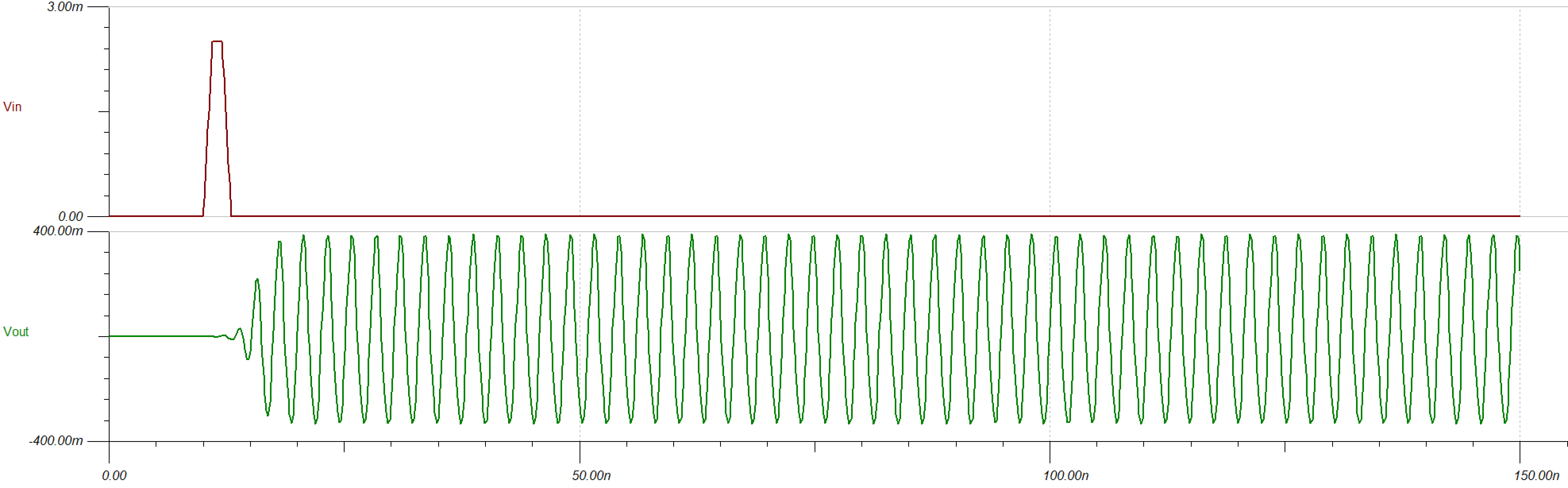
In analog electronic classes we’ve learned some amplifier systems like inverse proportionality converter, analog integrator, etc. The teacher must have mentioned about “feedback” and tell you that feedback in amplification systems is to restrict the differential signals in the linear region. However, when you build an amplification system in reality, especially for high frequency cases, you may encounter a very annoying phenomenon: oscillation. In an oscillting amplifier system, even if you do not apply any signals on the input terminal, the oscilloscope can detect signals at the output terminal, with unignorable amplitude. Typically, the output is a sinusoidal. This phenomenon is called “self-oscillation.”
You can see it in TINA TI simulator.
This phenomenon suggests that there must be more non-ideal effects should be taken into consideration. In practice, we should analyze the transfer function and modify it with extra components.
2. Oscillation Conditions
We know that an op-amp has large open-loop gain. So feedback is introduced to config the desired gain. Typically, an op-amp system can be decomposed into two parts: Gain net and feedback net.
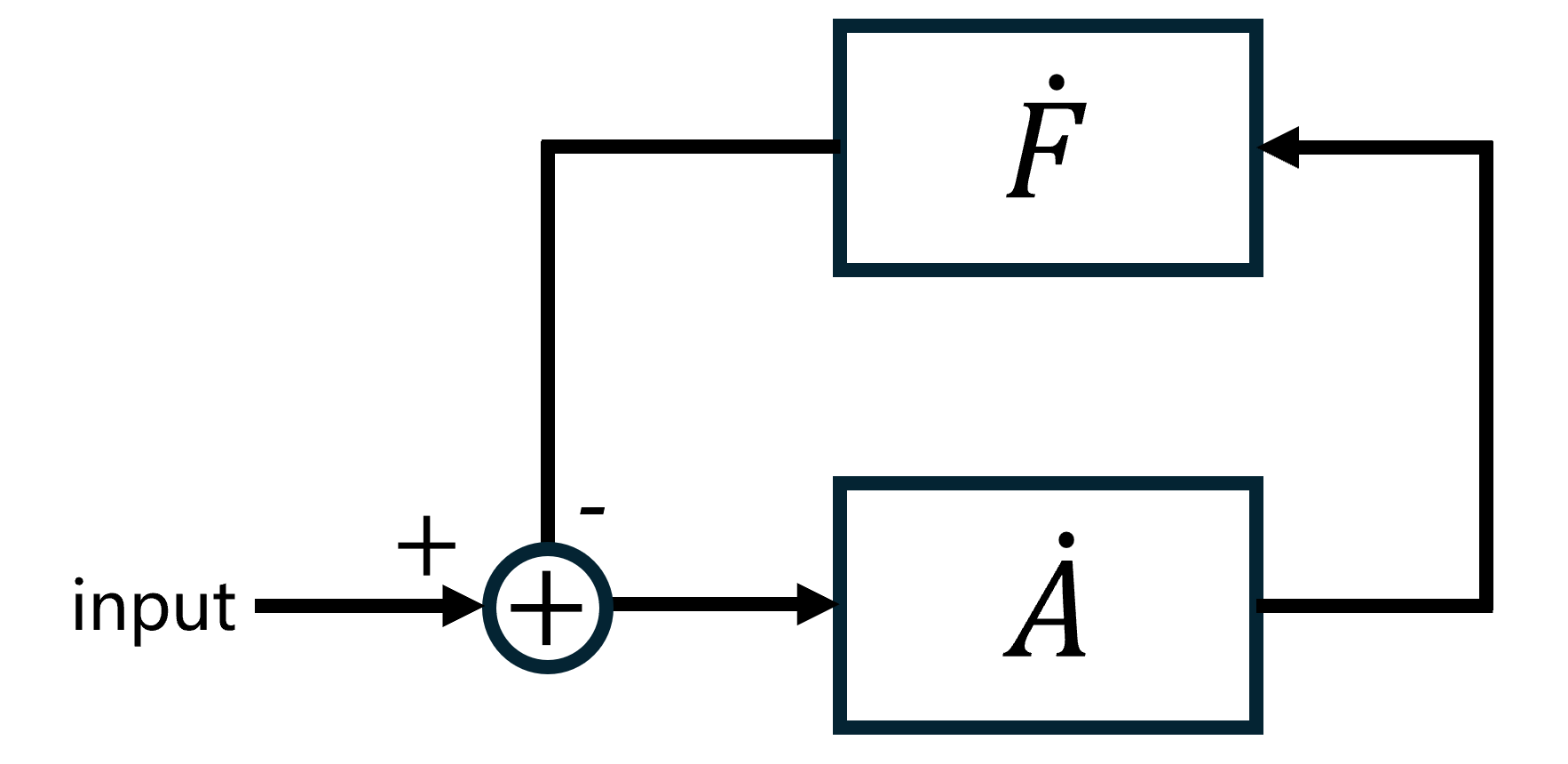
Now let’s make the signal path clear: A signal with only one freuqency component
Then it goes into the feedback network, scaled
This signal will be subtracted from the new input and re-enter the loop, repeating the entire process. Now we suppose the original input is an ideal pulse, which means when the signal completes one circle, the new input is 0. Generally the new input is
If
But the network parameters cannot be so precise in engineering. In practice the amplitude usually satisfies
Therefore, to avoid oscillation, we must violate the Barkhausen condition. At the frequency point where
3. Non-ideal Effects
3.1 Poles inside Op-amps
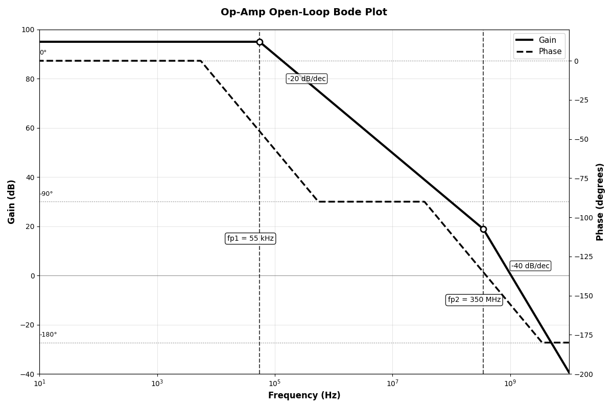
In engineering, op-amps are obviously not ideal. Op-amps are composed of basic components like resistors, capacitors and MOSFETs. These basic components, in conjunction with parasitic parameters, cause the op-amp itself to possess several poles. Currently op-amps in the market works under GHz level. In such frequency range we ususally take two poles into consideration. The first (with lower frequency) is called dominant pole, while the second is just called second pole. With poles in the op-amp taken into consideration, the open-loop gain becomes a function relative to frequency.
where
The open loop gain is then
Thus, with the frequency increasing, the gain decays and the phase shift reaches
The amplitude gain between
Obviously, when the frequency increases by a factor of 10, the open-loop gain decreases by 20 dB, denoted as -20dB/dec decay. That means a pole can cause a -20dB/dec decay on amplitude and -90° phase shift at most. At the pole frequency, the amplitude is -3dB(
When you encounter the second pole at higher frequency, it will bring the same effect. With the original -20dB/dec and -90° phase shift, the second pole worsen the gain to -40dB/dec and -180° phase shift.
In general, the manufacturer provides you the amplitude/phase - frequency curve with the datesheet. You can see the two poles on it clearly.
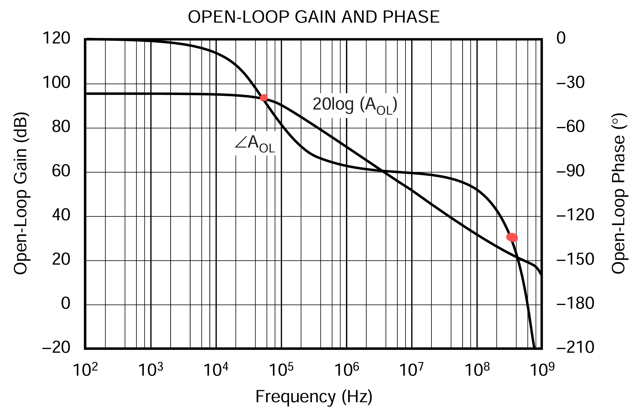
This figure is called Bode plot.
3.2 Unitary-Stability
Not all op-amps are unitary stable. I mean, if you configure the total gain as 1 (follower), it must oscillate no longer what measurement you apply to prevent it. Why? Let’s take a in-phase follower for example. Suppose the op-amp is OPA847, the Bode plot in the last section
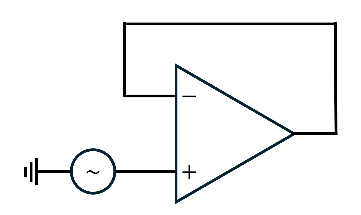
Let’s consider the single frequency signal,
- Enter op-amp from inverse phase terminal, amplitude 20dB, phase shift -180°-180°=-360° (extra -180° caused by “inverse phase”)
- Return to inverse phase terminal, amplitude 20dB, phase shift -360°
- Repeat these steps
When the test signal returns to the inverse terminal, its phase recovers to its original state, forming a positive feedback. Besides, 20dB > 0 so the amplitude increases. According to Barkhausen condition, it must oscillate.
Then consider a more general amplifier
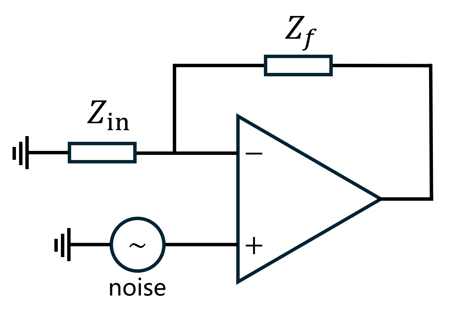
We equate all noise to the in-phase terminal and no other sources. Evidently the output is completely cause by noise and the noise gain is
In fact
The loop gain (NOT the total gain
Thus in Bode plot the loop gain equals to the open-loop gain minus noise gain. The key to stability is to keep the phase margin positive at the crossover frequency
You may discover that there is a gain require in the op-amp datasheet. For example OPA847 requires the gain to be at least 12 V/V. This means, under more than 12 V/V total gain, the phase margin is positive.
We have two methods to judge whether the op-amp is unitary stable:
- At the frequency where phase shift = -180°, if open-loop gain is more than 0dB, it is not unitary stable.
- At the frequency where open-loop gain = 0dB, if phase shift is worse than -180° (like -210°), it is not unitary stable.
You do not need to calculate
3.3 Input Impedance
The input terminal is also not ideal. For the op-amp itself, there is a differential capacitance
4. Feedback Compensation
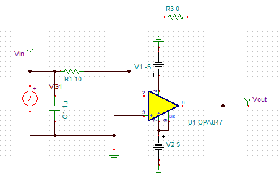
4.1 Transient Impedance Amplifier (TIA)
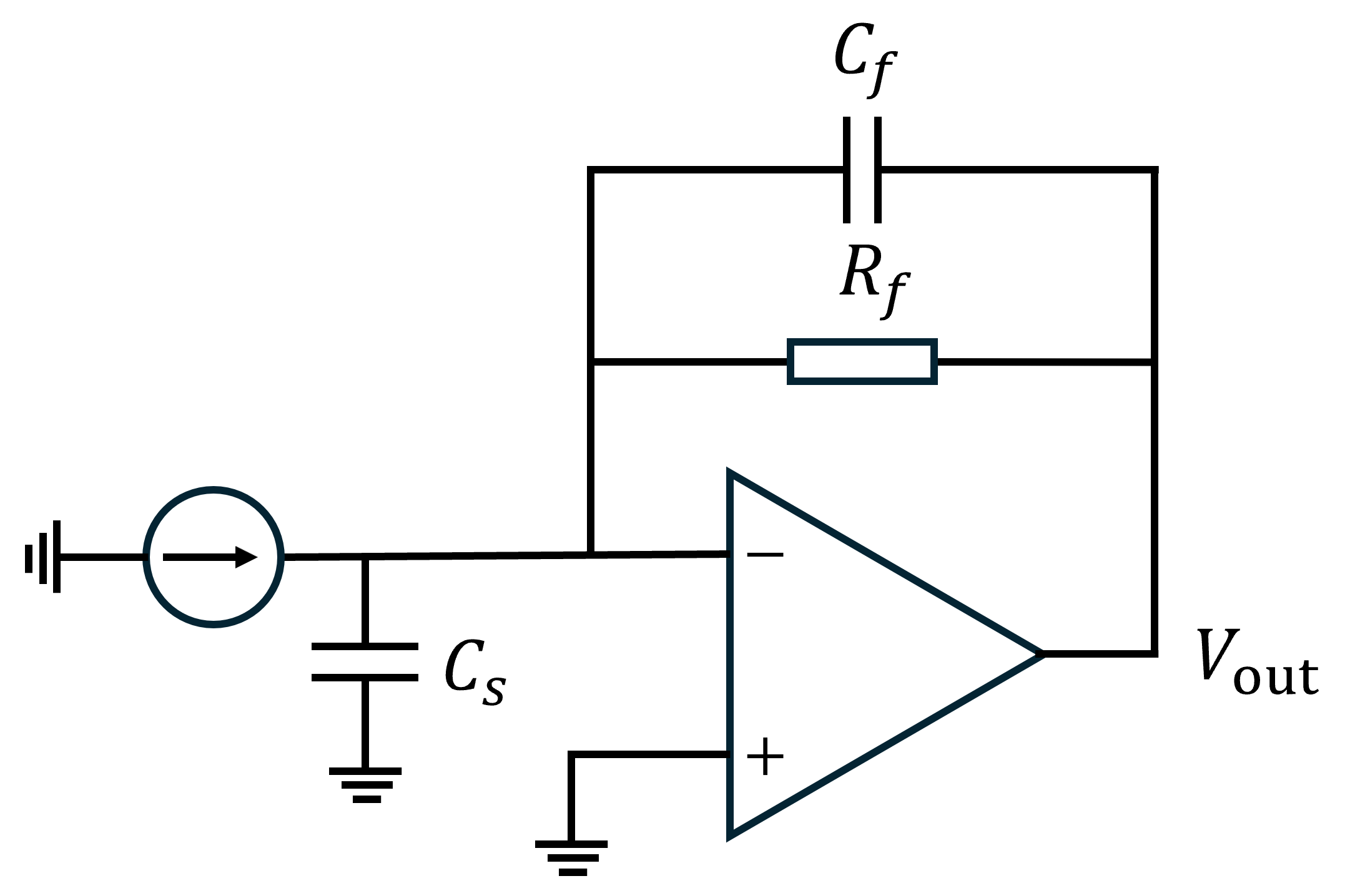
Transient impedance amplifier is a type of amplification system that transfer current signal into voltage signal. It is widely used in photoelectric detection. A fundamental inverse configuration is below.
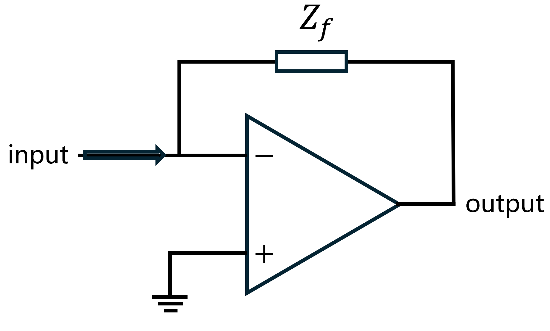
Ideally the output is
Suppose the
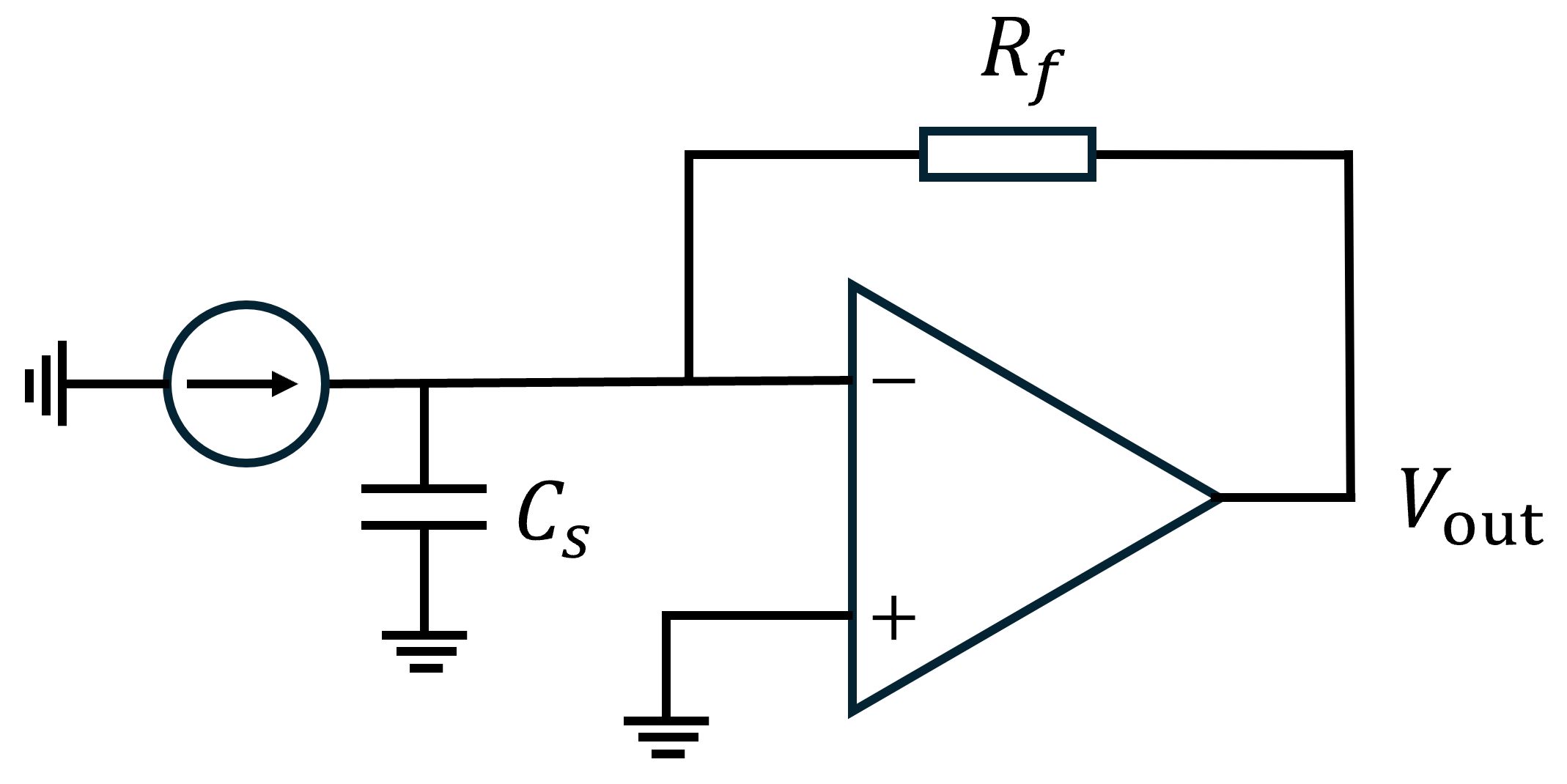
The feedback coefficient is
Suppose
The noise gain
We usually simplify the annoying curve to broken line. The line is broken at poles and zero points.
Add the noise gain curve. (Effects of zero points are opposite to pole points. Zero points introduce +45°, finally +90° phase shift and +20dB/dec amplitude increase.)
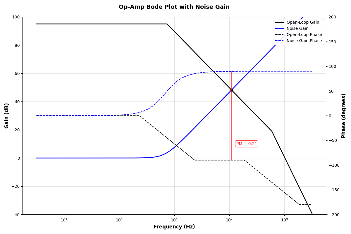
The phase margin is the difference between the noise phase shift and the op-amp’s phase shift, minus -180°. Clearly, with this parameter configuration, the phase margin is a mere 0.2°, meaning this circuit will almost certainly self-oscillate and fail to amplify current signals properly, especially in high frequency cases.
4.2 Calculation of Compensation Values
To resolve this problems we should take some measures to increase phase margin. Since the op-amp cannot be modified from PCB level, we have to modify the feedback network. Note that the deterioration of phase margin is caused by the zero of noise gain. So one idea is to introduce a pole to pull the phase shift back to -45°, and the phase margin will be fine. The simplest way is to parallelize a small capacitor
With this compensation, the new
Now a new pole point is introduced. Since in our cases
The new curve becomes
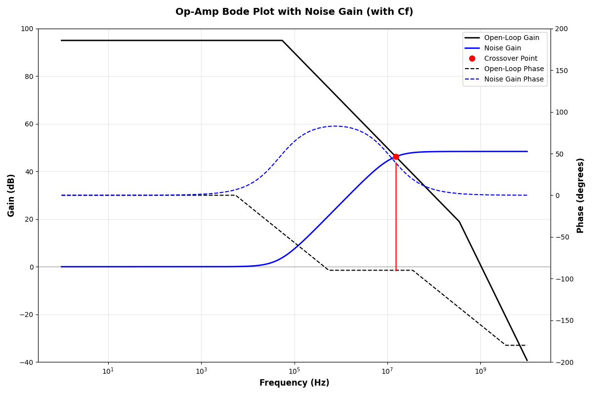
From the plot, to obtain a phase margin more than 45°, the pole point should be smaller than the crossover frequency.
At low frequency region, the open-loop gain can be represented by gain-bandwidth product (GBP)
At the crossover frequency
The approximation holds because
The pole is required
We get
This means the system can remain stable only when the compensation capacitor is over 11.8pF.
On the other hand, the capacitor cannot be too large, for it can influence your bandwidth. Generally, if we need a bandwidth of
If we need 5MHz bandwidth, the capacitor should be
Besides, OPA847 requires a gain over 12 V/V for stability. Check the noise gain curve. At high frequency region, impedance is dominant by the capacitance. Thus the high frequency gain is
But usually, the compensation range is determined by the two inequations:
References:
[1] Texas Instruments, Transimpedance Considerations for High-Speed Amplifiers, Application Report SBOA122, Nov. 2009.
[2] S. Cherian, What You Need to Know about Transimpedance Amplifiers - Part 1, Texas Instruments, Technical Article, 2023.
[3] Texas Instruments, Wideband, Ultra-Low Noise, Voltage-Feedback OPERATIONAL AMPLIFIER with Shutdown, Datasheet SBO251E, Dec. 2008
[4] 杨建国,《新概念模拟电路》. [Online]. 亚德诺半导体技术(上海)有限公司授权,2018.