Thermodynamics and Statistical Mechanics

Copyright Notice:
This article is licensed under CC BY-NC-SA 4.0.
Licensing Info:
- Title: Thermodynamics and Statistical Mechanics
- Author: EleCannonic
- Link: https://elecannonic.github.io/categories/physics/thermo/
Commercial use of this content is strictly prohibited. For more details on licensing policy, please visit the About page.
Part I. Macroscopic Thermodynamics
1.1 Equilibrium State and State Parameters
1.1.1 Equilibrium State
Thermodynamic equilibrium represents a fundamental state where a system's macroscopic properties remain constant over time without external influences. This static appearance masks intense microscopic activity - molecules continue moving and colliding, but their collective behavior produces stable macroscopic averages. A critical distinction exists between true equilibrium and steady states: while both show constant properties, steady states require continuous energy/matter exchange with surroundings, like a metal rod maintaining temperature gradient between 0°C and 100°C endpoints. True equilibrium demands three simultaneous conditions: thermal uniformity (no temperature gradients), mechanical uniformity (no pressure gradients), and chemical uniformity (no composition gradients). State parameters quantify these equilibrium properties. Volume1.1.2 Temperature
The zeroth law of thermodynamics provides the rigorous foundation for temperature's existence. Consider three systems A, B, and C. When A and C achieve thermal equilibrium, their state parameters satisfy:1.1.3 State Equation
The state equation- Boyle’s law (
at constant ) establishes isothermal compressibility - Gay-Lussac’s law (
at constant ) defines volume expansion coefficient - Charles’s law (
at constant ) gives pressure coefficient The ideal gas equation synthesizes these observations with Avogadro's principle. Starting from Boyle's law , consider a constant-pressure process with triple-point reference: Combining with Boyle's law at triple point yields: Avogadro's law confirms that is identical for all gases at given moles , defining universal constant : where is molar volume at triple point.
1.2 Microscopic Model of Matter
1.2.1 Introduction
The foundation of molecular kinetic theory lies in understanding matter at its most fundamental level. All macroscopic substances - whether solids, liquids, or gases - consist of vast numbers of microscopic particles called atoms or molecules, separated by empty space. This atomic structure explains why materials can be compressed: the apparent solidity of matter is an illusion created by electromagnetic forces between particles, not actual contact between them. Modern scientific instruments like scanning tunneling microscopes have made this invisible world visible, allowing us to image individual atoms and even manipulate them into structures like letters or patterns. The ceaseless, chaotic motion of these particles forms the heart of thermal phenomena. This motion intensifies with temperature, as dramatically demonstrated by Brownian motion - the random dance of pollen grains or smoke particles suspended in fluid. When observed under a microscope, these particles jitter unpredictably due to unbalanced collisions with surrounding fluid molecules. The smaller the particle, the more violent its motion becomes, providing direct evidence that what we perceive as "still" liquid or gas is actually a frenzy of molecular activity. This perpetual motion isn't confined to fluids; even in solids, atoms vibrate around fixed positions like springs connecting a molecular scaffold. Interactions between molecules govern material states through competing forces. At extremely close range (<0.1 nm), strong repulsive forces dominate as electron clouds overlap, preventing matter from collapsing into infinite density. At intermediate distances (0.1-1 nm), attractive forces take over through electromagnetic interactions between temporary dipoles in otherwise neutral molecules - the van der Waals forces that give liquids cohesion. These opposing forces create an equilibrium distance where molecules naturally settle, like dancers maintaining personal space in a crowded room. The delicate balance between molecular motion and these interaction forces explains phase transitions: heating provides kinetic energy to overcome attraction, turning solids to liquids to gases.1.2.2 Pressure of Ideal Gases
To understand gas pressure at the molecular level, we construct a simplified model that captures essential behaviors while ignoring complex details. Imagine gas molecules as infinitesimal points rather than physical objects - a reasonable approximation since molecular diameters (~10⁻¹⁰ m) are dwarfed by typical intermolecular separations (~10⁻⁹ m at STP). Between collisions, these particles move freely without mutual attraction or repulsion, like commuters ignoring each other in a vast train station. Collisions between molecules or with container walls occur instantaneously and elastically, conserving both momentum and kinetic energy like perfect billiard ball impacts. This idealization emerges naturally from experimental observations: gases expand to fill containers because molecules move independently; low densities make compression easy by reducing intermolecular distances; constant pressure at equilibrium implies steady collision rates. The model's power lies in transforming the chaotic complexity of 10²³ molecules into tractable statistics, where individual paths become irrelevant and collective averages dominate.1.2.3 Statistical Assumptions at Equilibrium
When gas reaches thermodynamic equilibrium, two powerful statistical principles emerge despite ongoing molecular chaos. First, molecules distribute uniformly in space - any macroscopic volume element contains approximately equal particle numbers regardless of location. This spatial homogeneity allows defining number density1.2.4 Ideal Gas Pressure Formula
Pressure emerges from the relentless barrage of molecular impacts on container walls. Consider molecules approaching a wall area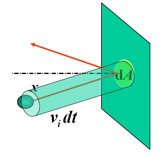
1.2.5 Microscopic Interpretation of Temperature
Connecting microscopic motion to temperature starts with combining the pressure equation1.2.6 Molecular Forces
Beneath the apparent simplicity of gases lies a complex interplay of electromagnetic forces. Each molecule contains positively charged nuclei surrounded by negatively charged electrons. When molecules approach, their electron clouds distort, creating temporary dipoles that generate attractive forces - the van der Waals interaction. At closer ranges, Pauli repulsion dominates as overlapping electron orbitals resist compression. These competing effects produce the characteristic molecular force curve: strongly repulsive below equilibrium distance- Lennard-Jones potential:
balances short-range repulsion (r⁻¹² term) with longer-range attraction (r⁻⁶ term). The minimum at represents optimal bonding distance. - Sutherland potential:
models impenetrable hard spheres with weak attraction. - Hard-sphere potential:
ignores attraction entirely, focusing on excluded volume effects. These models serve different purposes: Lennard-Jones accurately describes noble gases, Sutherland simplifies van der Waals theory, while hard-sphere models help understand dense fluids.
1.2.7 Pressure in van der Waals Gases
Real gases deviate from ideal behavior through two molecular effects: finite size and mutual attraction. Johannes van der Waals ingeniously modified the ideal gas law to account for both. First, molecules occupy physical space, reducing the available volume for motion. For1.3 Distribution of Molecular Speeds and Energy
1.3.1 Maxwell’s Speed Distribution Law
The molecular speed distribution in an ideal gas at thermal equilibrium is derived from fundamental statistical principles. Consider the velocity distribution function1.3.2 Characteristic Speeds and Distribution Properties
The most probable speed1.3.3 Boltzmann Distribution in Force Fields
In conservative force fields, the Maxwell distribution generalizes to the Boltzmann distribution. For a potential energy1.3.4 Equipartition Theorem and Energy Distribution
The equipartition theorem states: each quadratic term in a system's Hamiltonian contributesTranslational: 3 terms
→ Rotational: 2 (diatomic) or 3 (polyatomic) terms →
or Vibrational: Kinetic and potential terms each contribute
per mode For a diatomic molecule, total energy is (rigid) or (non-rigid). Molar heat capacity at constant volume is: where is the number of quadratic degrees of freedom.
1.4 Mean Free Path of Gas Molecules
1.4.1 Mean Collision Frequency and Mean Free Path
Gas molecules move at high thermal speeds (e.g., nitrogen at 27°C averages 476 m/s), yet macroscopic diffusion occurs slowly due to frequent collisions that randomize molecular paths. The mean free path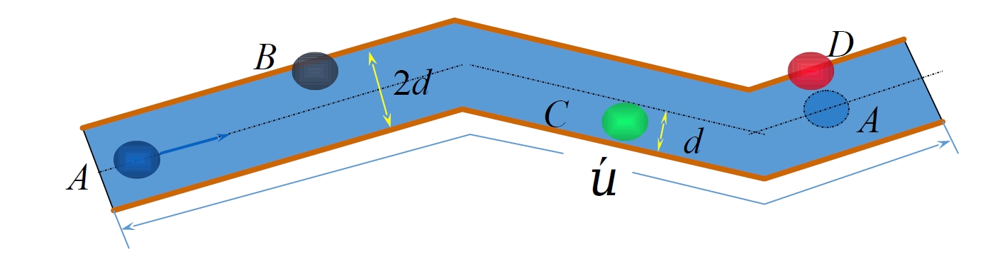
1.4.2 Distribution of Free Paths
The probability that a molecule travels distance1.4.3 Viscosity
When adjacent fluid layers move at different velocities (e.g.,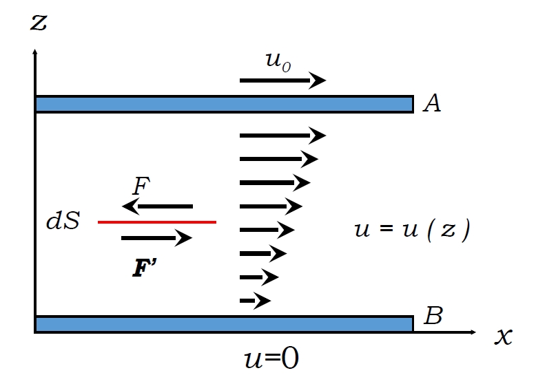
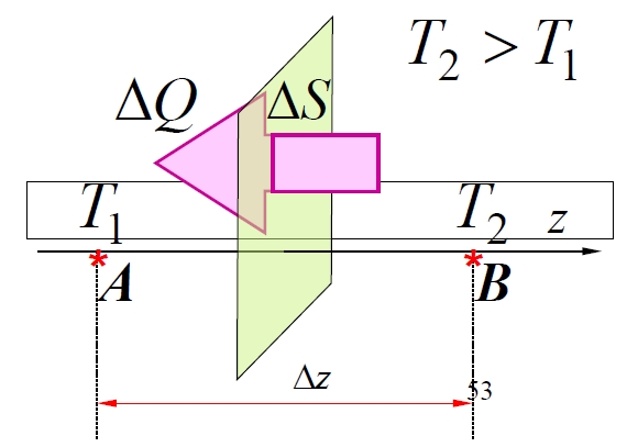
1.4.4 Heat Conduction
Heat conduction occurs when temperature gradients exist. Fourier's law describes the heat flux- In region A:
(for translational energy; for molecules with degrees of freedom, it's , ) - In region B:
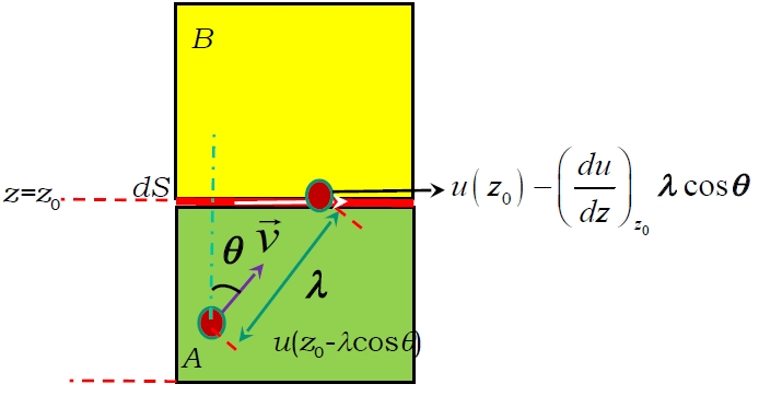
, The number of molecular pairs exchanged across an area in time is estimated as: (The factor arises from considering the fraction of molecules moving perpendicular to the surface in a specific direction within an isotropic gas). The net energy transported along the positive z-axis per exchanged molecular pair is the difference: The total energy transported through along the positive z-axis in time (i.e., the heat ) is: The temperature difference is related to the temperature gradient at : Substituting this in: Comparing this to Fourier's law , the thermal conductivity is identified as: Using the molar heat capacity at constant volume (where is Avogadro's number), and the specific heat capacity (per unit mass), and the density , this can be rewritten as: 
Demonstration of Heat Conductance
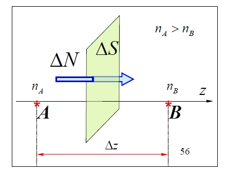
1.4.5 Diffusion
Diffusion transports mass due to density gradients. Fick's law for the mass| Gas | ||
|---|---|---|
| Gas 1: Hydrogen ( |
3 | 0.594 |
| Gas 2: Carbon Dioxide ( |
1 | 0.605 |
1.5 The First Law of Thermodynamics
1.5.1 Thermodynamic Processes
A thermodynamic process, or simply process, occurs when the state of a system changes over time. For example, when advancing a piston compresses gas in a cylinder, the gas's volume, density, temperature, or pressure will change, and at any moment during the process, the density, pressure, and temperature are not identical throughout the gas. Thermodynamic processes are classified into non-quasistatic processes and quasistatic processes. In non-quasistatic processes, the system transitions from an equilibrium state to a disrupted state before reaching a new equilibrium. The time from equilibrium disruption to new equilibrium establishment is called relaxation time (1.5.2 Work
Work is a method of energy exchange. In thermodynamics, it represents the conversion between ordered mechanical energy from the surroundings and disordered thermal energy of the system, denoted as1.5.3 Heat
Heat is another method to change system state, distinct from work. While work involves energy transfer through generalized forces causing generalized displacements, heat transfer occurs due to temperature differences. Joule's experiments demonstrated that heat production or disappearance always accompanies equivalent disappearance or production of other energy forms (mechanical, electrical), proving no separately conserved "caloric" exists. Instead, heat, mechanical energy, and electrical energy together conserve energy. Heat (1.5.4 The First Law of Thermodynamics
Joule's experiments revealed a definite equivalence between heat and work (1 cal = 4.186 J), showing interconversion between mechanical/electromagnetic and thermal motion. This led to the energy conservation and transformation law: all matter possesses energy in various forms convertible between each other and transferable between objects, with total quantity conserved. An alternative statement: perpetual motion machines of the first kind are impossible. For a system changing from initial state 1 to final state 2 via an adiabatic process (no heat exchange), the work done by surroundings is the adiabatic work. Joule's experiments showed that for fixed initial (state 1, temperature1.5.5 Heat Capacity and Enthalpy
Heat capacity1.5.6 Internal Energy of Gases and Joule-Thomson Experiment
In Joule's 1845 free expansion experiment, gas expanded into vacuum with no temperature change observed. Applying the first law (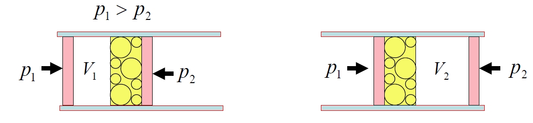
Process Applications:
Isochoric (
constant): , , , . Isobaric (
constant): Isothermal (
constant): , , . Adiabatic (
): , leading to , , . Work . For a polytropic process , the molar heat capacity is derived from the first law and process equation. For 1 mole of ideal gas: The molar heat capacity is defined as , so: From the polytropic equation and ideal gas law , solve for : Differentiate with respect to : Rearrange to express : Substitute: Thus: Using and , express as: Substitute into (2): Solving for in terms of heat capacities:
Then special cases can be verified:
Isobaric (
): Isochoric (
): (limit of ) Isothermal (
): (undefined, consistent with ) Adiabatic (
): (since )
1.5.7 Cyclic Processes and Carnot Cycle
Cyclic processes involve a working substance returning to its initial state after completing a series of thermodynamic changes. Quasistatic cycles are represented as closed curves on P-V diagrams, with clockwise cycles functioning as heat engines and counter-clockwise cycles as refrigeration systems. In heat engines, the working substance absorbs heat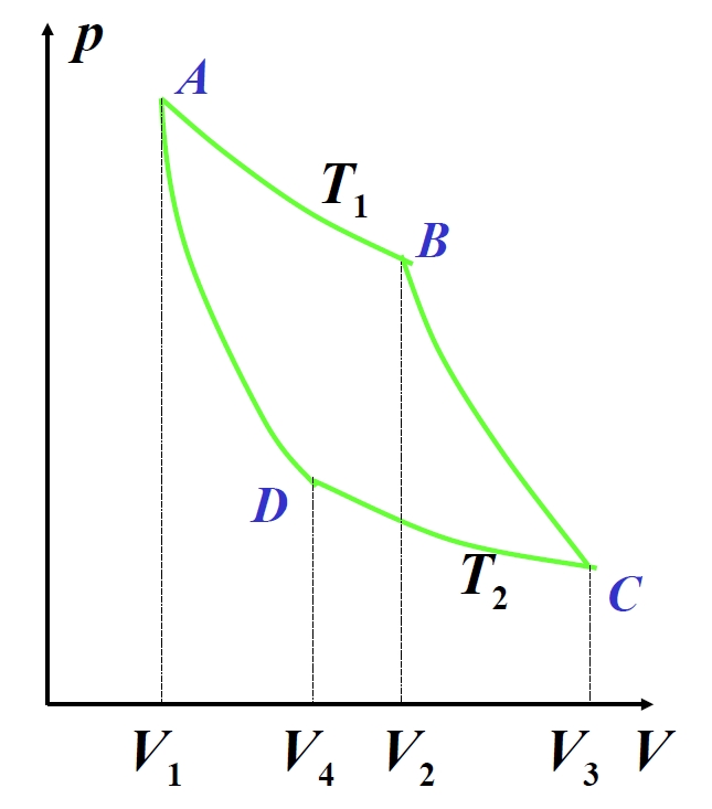
The Carnot cycle—a fundamental model for heat engines—combines two isothermal and two adiabatic processes. For an ideal gas working substance:
Isothermal expansion (A→B):
Adiabatic expansion (B→C):
Isothermal compression (C→D):
Adiabatic compression (D→A):
The adiabatic equations yield the volume ratio relationship: Substituting into the efficiency formula: This result depends solely on reservoir temperatures and is independent of the working substance.
Practical engine implementations also include:
- Otto cycle (constant-volume heating) with efficiency:
where is the compression ratio. - Diesel cycle (constant-pressure heating) with higher efficiency due to greater compression ratios.
1.6 The Second Law of Thermodynamics
1.6.1 The Second Law of Thermodynamics
The Second Law of Thermodynamics addresses the directionality of natural processes, complementing the First Law's energy conservation principle. While the First Law prohibits perpetual motion machines of the first kind (violating energy conservation), it does not restrict process directionality. For example, heat spontaneously flows from high to low temperatures but not the reverse. The Second Law resolves this through two equivalent formulations:- Kelvin Statement (1851): It is impossible to convert heat entirely from a single heat source into work without other effects. This implies heat engines cannot achieve 100% efficiency (
) and prohibits perpetual motion machines of the second kind. - Clausius Statement (1850): Heat cannot spontaneously flow from a cold to a hot body without external work input. This establishes the directional nature of heat transfer and limits refrigeration efficiency (
).
We now prove the equivalence between Kelvin and Clausius Statements:
(1) Clausius false ⇒ Kelvin false
Assume device(2) Kelvin false ⇒ Clausius false
Assume device1.6.2 Carnot Theorem
Carnot Theorem establishes the theoretical limits for heat engine efficiency operating between thermal reservoirs at temperatures1.6.3 Thermodynamic Temperature Scale
The thermodynamic temperature scale, established by Lord Kelvin using Carnot's Theorem, provides a universal temperature definition independent of material properties. For a reversible heat engine operating between reservoirs at empirical temperatures1.6.4 Entropy
The Second Law of Thermodynamics addresses the directional nature of natural processes, complementing the First Law's energy conservation principle. Kelvin's statement (1851) declares it impossible to convert heat entirely from a single source into work without other effects, implying heat engines cannot achieve 100% efficiency (Part II. Classical Statistical Mechanics
Note:
Before you read this part, please make sure you have learned Classical Mechanics, Quantum Mechanics and Probability.
In Part II and Part III, Boltzmann constant are all normalized to
. So temperature and energy have the same unit.
2.1 Description of States
Statistical physics connects the behavior of individual particles to the measurable properties of materials
we observe in everyday life.
To understand how this connection works,
we first need a way to describe the detailed state of a many-particle system.
Consider an isolated system composed of
like molecules in a sealed container.
Each particle requires six numbers to fully specify its mechanical state:
three position coordinates
For the entire system,
we must account for all particles simultaneously.
The complete microscopic state - called a microstate - is therefore described by listing all positions and momenta together:
This collection of
Classical mechanics demonstrates that if we know this phase space point at any instant,
and the system’s Hamiltonian
we can in principle determine its future evolution through Hamilton’s equations:
Thus, a single point in phase space completely defines the instantaneous mechanical state of the entire system.
However, for macroscopic systems where
tracking individual phase space points becomes fundamentally impossible.
Moreover, laboratory measurements of quantities like pressure or temperature inherently average
over enormous numbers of microstates - approximately
This practical limitation necessitates a shift from deterministic mechanics to probabilistic description.
Rather than following exact trajectories,
we must consider how microstates are distributed throughout phase space,
leading us to the core methodology of statistical physics.
Based on this description, we must specify the characterization of the macro-system.
For an isolated system (no exchange of particles and energy with the environment),
its macro-state can be completely determined by 3 measureable conservation quantities:
Number of particles
Volume of the system
Energy of the system
Why these three? Macroscopic measurements cannot distinguish microstates sharing same
Hence, parameters
Such a macro-state contains a massive number of micro-states. It corresponds to a set in the phase space:
The condition
defines a
which causes difficulty for calculation of probability.
To solve this problem, we need to introduce energy shell.
Based on the hypersurface, we extend another dimension to give it a small “thickness”
Then, the hypersurface turns into a thin space, represented by:
This extended space is called a energy shell.
Note that
but it’s necessary to include sufficient microstates (
With a dimension of
we can calculate the probability in the phase space.
We can figure out the “volume” of the energy shell:
where
The volume describes the number of micro-states in
2.2 Boltzmann Postulate
Initially, researchers tried to establish connections between macro and micro states by ergocity assumption.
They think isolated systems traverse all reachable states on an energy hypersurface for a sufficiently long time.
However, time scale required for strict traversal is far more larger than the age of the universe,
so it’s impossible in measuring.
To solve this problem, Boltzmann raised the most postulate in statistical mechanics:
Boltzmann Postulate: For an isolated system under equilibrium, all micro-states have equal probability.
Equilibrium means all observable properties (e.g., temperature, pressure, density) are time-invariant and uniform in space.
Based on this postulate, we can figure out the probability of a microstate in an energy shell:
where
Almost everything in statistical mechanics is established on the Boltzmann’s postulate.
2.3 Entropy
2.3.1 Gibbs-Shannon Entropy
Since macroscopic measurement cannot distinguish microstates,
while one macrostates include massive microstates,
we need a quantity to quantify the scale of indistinguishability.
Imagine you are predicting the weather tomorrow:
If it is known that tomorrow will definitely be sunny
(
there is no doubt about the outcome of the prediction and the uncertainty is zero.
When you learn that it will be sunny,
the amount of information you get is also almost zero (you already knew).
If the probability of it being sunny or rainy tomorrow is 50/50
(
the prediction is most uncertain. You get the most information
(eliminating the most uncertainty)
when you learn that it will be sunny (or rainy).
If the probability of tomorrow being sunny is 0.9 and rainy is 0.1,
the uncertainty is somewhere in between.
Learning that it will be sunny brings less information (expected)
and learning that it will be rainy brings more information (unexpected).
From the example above,
it’s clear that information carried by the events is
strongly related to the probability distribution.
Generally, we can define a function
This function should satisfy the conditions below:
is continuous - If an event occurs with probability
, - For independent events
, ,
We now derive the explicit form of
In terms of probabilities,
letting
we have the functional equation:
Define
From the conditions,
We assume that
This assumption is justified because the continuity of
and the functional equation imply that
(as is standard in solving Cauchy functional equations).
Fix an arbitrary
Consider the functional equation as a function of
Differentiate both sides with respect to
(treating
as constant):
Left side:
by the chain rule. Right side:
,
sinceis constant with respect to .
Thus:
Solving for
Equate the expressions for
Rearranging:
Equation (*) holds for all
Since the left side depends only on
both sides must equal a constant,
say
Therefore:
where
Solving for
Integrate both sides with respect to
where
Apply the condition
Since
we have
Now apply the condition
For
so to ensure
we must have
Let
Then:
This is equivalent to:
since any logarithm base can be absorbed into the constant
(as
so
Now we have proved
Returning to the context of microstates, we can define Gibbs-Shannon entropy:
where
The Gibbs-Shannon entropy reflects the uncertainty and disorder of a thermodynamic system.
2.3.2 Boltzmann Entropy
After Gibbs-Shannon entropy, we can define another type of entropy called Boltzmann entropy.
where
We can find that when
So Boltzmann entropy is a special case of Gibbs-Shannon entropy at equilibrium.
By the way, Boltzmann entropy is only defined at equlibrium,
while Gibbs-Shannon entropy can also be defined at non-equilibrium.
2.3.3 Maximal Entropy Principle
Boltzmann’s postulate of equal probability leads to the principle of maximum entropy:
The Gibbs-Shannon entropy of an isolated thermodynamic system is maximized at equilibrium.
The process of converging to equilibrium is a process of increasing entropy.
There is a proof:
The equals sign is taken when
This principle means equilibrium states gives maximum entropy.
By the thermodynamics 2nd law, any isolated systems tend to evolve towards equilibrium state.
2.4 Ensembles
An ensemble in statistical mechanics is a probability
distribution over the system’s phase space, representing our knowledge (or
ignorance) of the system’s exact microstate.
2.4.1 Micro-canonical Ensemble
The microcanonical ensemble is the starting point of equilibrium statistical
mechanics. It describes an isolated system —one that can exchange
neither energy, volume, nor particles with its surroundings —and assigns
probabilities to its microscopic states.
In classical mechanics, the state of a system of
in a box with volume
the
But thermodynamics makes no reference to microstates —
it deals only with macroscopic variables such
as energy
The goal of statistical mechanics is to explain thermodynamics as a consequence of statistical
properties of microscopic degrees of freedom.
Recall the energy shell
instead of the characteristic function
we can also represent it with delta function:
where
is referred to as the “surface area” of the constant energy surface.
In the microcanonical ensemble, the fundamental thermodynamic quantity
is the Boltzmann entropy (at equilibrium), which is defined as
The factor on the denominator is to elliminate quantum effects.
We can rewrite the entropy:
It is obvious that
and
whereas
Hence in the thermodynamic limit,
we may ignore
and have
In thermodynamics, all state variables can be derived from the fundamental
relation
It is useful to think of this function as a surface in a four dimensional space spanned by
This surface was called the fundamental surface by Callen.
The microcanonical ensemble realizes this idea concretely by connecting entropy to the volume of phase space.
Once we have the entropy as a function of energy, volume, and particle number,
we can define all other thermodynamic quantities as its partial derivatives.
Temperature
Temperature measures how rapidly the number of accessible microstates increases with energy.
For the temperature to be well-defined and positive,
the function
Physically, this is almost always true for large systems —
higher energy means more ways to distribute that energy among microscopic degrees of freedom.
Pressure
Pressure arises from the fact that increasing the volume allows more microstates
to be accessible —especially if particles are free to move. Thus,
the entropy increases with volume, and this increase (scaled by temperature)
defines the pressure exerted by the system. However, negative pressure
is not a signature of thermodynamic instability.
If the number of particles
chemical potential
This expresses how the entropy changes when a particle is added to the system,
at fixed energy and volume.
It is especially important when studying systems that can exchange particles (grand canonical ensemble),
but the definition remains valid even in the microcanonical ensemble as a formal identity.
To recap, we can reassign these definitions:
reassign again:
This is in fact the 1st thermodynamics law.
And it’s easy to extend all the things in this section above to multi-component systems.
Just extend
Let’s take the ideal gas in micro-canonical ensemble for example:
Consider a classical ideal gas of
confined to volume
The Hamiltonian is purely kinetic:
The surface area
Integrate over coordinates (yields
Set
Using the surface area of a
For
Apply Stirling’s approximation for large
Retain extensive terms:
This is the Sackur-Tetrode entropy.
Scale variables by
- Temperature:
- Pressure:
- Chemical potential:
2.4.2 Canonical Ensemble
Different from micro-canonical ensemble,
the canonical ensemble describes systems in thermal equilibrium with a heat bath at fixed temperature.
It allows variation of
which in micro-canonical fixed.
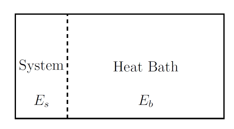
Consider a large, isolated system with total energy
If we divide the entire system into 2 parts: subsystem and reservoir,
the energy will be divided into 3 parts:
System: Small subsystem with Hamiltonian
Heat bath: Large reservoir with Hamiltonian
Interaction: Interaction between the system and the reservior
However, in large systems, interaction is extremely weak compared to interal actions.
So interaction Hamiltonian is neglected.
The system and reservoir exchange energy through a diathermal wall,
with fixed
By Boltzmann’s postulate, every microstate of the combined system has equal probability.
The total number of microstates is:
We split this integral by inserting
Now consider microstate
Given
but
There’re many
Hence, the probability density for the system to be in microstate
where
Since the bath is much larger than the system (
Define the inverse temperature:
Thus:
The proportionality constant defines the partition function:
giving the canonical distribution:
The probability density for the system to have energy
where
The partition function,
is an extremely important function in statistical mechanics.
(Partition function of micro-canonical ensemble is
It serves as the generating function for all thermodynamic properties of the system.
Let’s define free energy first:
is called the Helmholtz Free Energy.
Through Helmholtz free energy and partition function,
we can calculate almost all thermodynamics quantities.
Average Energy:
Gibbs-Shannon Entropy:
This result can derive the relationship between Helmoholtz free energy with energy:
Take derivative and plug result of
- Energy Variance:
We also have
Hence,
This shows equivalence with the microcanonical ensemble in the thermodynamic limit.
- The bath’s constant temperature
emerges from its large size - Rare high-energy states are exponentially suppressed by
- Free energy
encodes the competition between energy and entropy
2.4.3 Grand Canonical Ensemble
The grand canonical ensemble is almost the same as canonical ensemble
except that
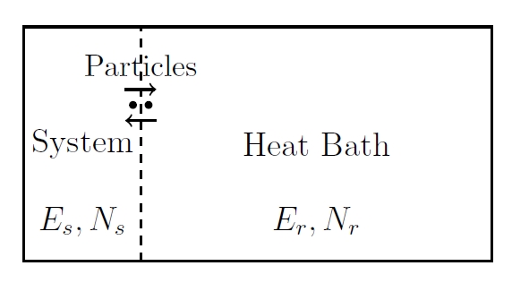
Imagine a large, isolated system characterized by its total energy
total particle number
and total volume
This overarching system can be described by its microcanonical partition function,
where
signifies integration over all possible microstates.
Now, consider dividing this isolated system into a small subsystem
(denoted by the subscript ‘s’)
and a vast reservoir (subscript ‘r’).
The total particle number is conserved,
meaning
The microcanonical partition function can then be expressed
as a sum over possible particle numbers in the subsystem
(
and an integral over possible energies in the subsystem (
The probability density of finding the subsystem with energy
and particle number
Here,
For a sufficiently large reservoir,
we can perform a Taylor expansion of its entropy around the total energy and particle number of the isolated system:
In this expansion,
and
Substituting this back into the probability density equation,
we arrive at a crucial expression for the probability density in the grand canonical ensemble:
The denominator,
This partition function effectively normalizes the probability.
The probability of a specific microstate (
of the subsystem with
The normalization condition,
allows us to express the grand canonical partition function in terms of the Hamiltonian
A remarkable aspect of the grand canonical ensemble is its direct relationship to the canonical ensemble.
The canonical partition function,
fixed volume
and fixed temperature
The grand canonical partition function can be seen as a sum over all possible canonical ensembles,
weighted by the factor
This equation elegantly demonstrates that the grand canonical ensemble is,
in essence, a statistical amalgamation of many canonical ensembles,
each corresponding to a different number of particles.
This formulation is particularly powerful for systems where particle number is not a conserved quantity.
Just as the Helmholtz free energy is derived from the canonical partition function,
the grand potential,
is defined from the grand canonical partition function:
The grand potential provides a direct link to the system’s thermodynamic properties.
From the Gibbs-Shannon entropy,
we can derive a fundamental relationship:
Rearranging this equation,
we find an important expression for the grand potential in terms of other thermodynamic quantities:
Here,
Differentiating the grand potential yields several crucial thermodynamic relations:
From this differential,
we can derive the following thermodynamic relations:
- Average Particle Number:
- Pressure:
- Average Energy:
From the first law of thermodynamics,
and the extensivity of energy (
we know that
Combining this with the definition of the grand potential,
leads to a remarkable identity:
This equation establishes a direct connection between the grand potential and the pressure-volume product of the system.
Furthermore, the Gibbs free energy,
can be shown to be equal to
This implies that the chemical potential
This relation highlights the interdependence of intensive variables
(temperature, pressure, and chemical potential).
On a per-particle basis, it can be written as:
where
is the entropy per particle and
A key aspect of the grand canonical ensemble is
its ability to describe fluctuations in energy and particle number,
which are inherently allowed due to the system’s coupling with the reservoir.
The mean square fluctuations are defined as:
These fluctuations are directly related to derivatives of the grand canonical partition function:
- Particle Number Fluctuations:
- Energy and Particle Number Cross-Fluctuations:
For macroscopic systems,
these fluctuations scale as
and are therefore negligible compared to the average values,
which scale as
This means that for large systems,
the grand canonical ensemble’s predictions for average quantities
will converge with those from other ensembles.
However, the grand canonical ensemble remains invaluable
for understanding and calculating properties of open systems where particle exchange is crucial.
2.4.4 Recap
In the thermodynamic limit, where the particle number
Similarly, in the grand canonical ensemble, both particle number and energy fluctuations become negligible. Particle number fluctuations obey
Thus, the vanishing relative fluctuations and mathematical consistency of thermodynamic potentials establish the equivalence of the three ensembles for macroscopic systems.
2.5 Extremum Principles
2.5.1 Thermodynamic Potentials
We have known the energy
Helmholtz Free Energy
and grand potential
Operate a Legendre transformation,
This is defined as the Gibbs Free Energy.
Take a diffrential, we can get
We can also define Enthalpy:
What we must clarify is that
differential variables in the differential equation is the natural variable of that potential.
Take energy
we have
and we can expand this example to
For example we can say
2.5.2 Maxwell Relation
The thermodynamic potentials are well-defined single-valued functions of their natural variables.
In mixed second order derivatives such as
the order of partial derivative can be exchanged:
since
so we obtain:
This leads to a very large number of identities between partial derivatives
of various thermodynamic variables, all called Maxwell relations:
Since these differentials are exact, mixed partials yield Maxwell relations.
We list all 15 Maxwell relations below:
| Potential | Relations |
|---|---|
2.5.3 Extremum Principles
As we have already shown in Lect. 2, the equilibrium state of an isolated
system maximizes the Gibbs-Shannon entropy, subject to the constraints
of probability normalization and fixed energy (which means that the prob-
ability density function vanishes outside the energy surface). The entropy
maximizing probability distribution is an equal probability distribution on
the energy surface. Hence the maximal entropy principle is ultimately
equivalent to Boltzmann’s postulate of equal probability. Either can be
used as a starting point of equilibrium statistical mechanics.
Consider a system with continuous microstates
with fixed volume
Let
the probability density of an arbitrary non-equilibrium state.
The average energy is:
and the Gibbs-Shannon entropy is:
Define the non-equilibrium Helmholtz free energy as:
where
Introducing a Lagrange multiplier
The first variation,
which yields a canonical distribution:
The second variation,
At equilibrium, the non-equilibrium Helmholtz free energy
Note that this principle is valid for both small systems and large systems. It is straightforward to verify that this principle can also be reformulated in the following equivalent form:
At equilibrium, the Gibbs-Shannon entropy of a thermally open system is maximized subject to normalization and fixed average energy.
Now consider a system exchanging energy and particles with a bath at temperature
and Gibbs-Shannon entropy:
The non-equilibrium grand potential is defined as:
We seek
Using a Lagrange multiplier
Setting the functional derivative to zero:
we find the grand canonical distribution:
where
At equilibrium, the non-equilibrium grand potential
An equivalent representation of this extremum principle is the following:
At the thermodynamic equilibrium, the Gibbs-Shannon entropy of an open system is maximized subject to the constraints of probability normalization and fixed average energy, and fixed average particle number.
2.6 Equilibrium Conditions
2.6.1 Thermal Equilibrium
Consider an isolated system composed of two subsystems that can exchange energy
(This is in fact the canonical ensemble).
The number of accessible microstates for a given division of energy is:
and the corresponding probability is
According to the maximal entropy principle,
we need to maximize
To find the value of
maximizing
(denoted as
we should take the derivative:
This gives
Expanding
with
yields a Gaussian distribution
and the fluctuation
If
then the entropy change associated with a small energy
transfer
This indicates that entropy increases when energy flows from the hotter to the colder subsystem.
2.6.2 Mechanical Equilibrium
Now consider two subsystems that can exchange volume through a movable, frictionless piston,
while the total energy and total volume remain fixed.
Let subsystem 1 occupy volume
and subsystem 2 occupy
The total entropy is:
The most probable configuration maximizes the total entropy with respect to variations in
since
Assuming thermal equilibrium has already been established,
this simplifies to
This is the mechanical equilibrium.
The same as temperature,
we can derive such a relationship:
This aligns with the everyday notion of pressure as a force that drives expansion.
In equilibrium, the driving force vanishes; outside equilibrium, it
gives rise to directional motion that increases entropy. Hence, the common
physical interpretation of pressure as an expansive force is fully consistent
with its thermodynamic and statistical definitions
2.6.3 Chemical Equilibrium
The same, we can also derive chemical equilibrium.
Consider a system with multiple components, we have
Using the identity:
We have
Hence, particles flow spontaneously from higher to lower chemical potential,
just as heat flows from hot to cold and volume expands from high to low
pressure. The chemical potential can thus be interpreted as a generalized
”force” driving particle exchange toward equilibrium.
2.7 Stability Condition
2.7.1 Entropy Stability
Consider two systems with same macrostates
(i.e., same
According to the scaling property,
we have
Now apply small perturbations to the system:
Our target is to find the stability condition.
Recall that stability corresponds to second order derivative.
So we expand
The differential of the entropy for a single subsystem is:
We can take differential of these equations. Finallt get
Since entropy is maximized,
if we want the system to be stable,
Then
2.7.2 Diagonalization of
We can express the second variation of entropy as a quadratic form:
where
etc.
From the thermodynamic identity:
we can solve for
Substituting into
To simplify, define new coefficients:
and introduce a new variable
Suppose
We can derive a Jacobian determinant
Change variables to
Since
then we can find that
Substituding the results into
This requires two independent stability conditions:
2.7.3 Chemical Stability
We consider
Then second derivative reduces to
This leads to another stability condition:
Substitute:
So chemical stability leads to
2.8 First Order Phase Transition
2.8.1 Conflict at Transition Point
First-order phase transitions, such as boiling or melting, are marked by discontinuities
in thermodynamic observables—like energy or volume—as external
parameters like temperature or pressure are varied. These discontinuities signal
the coexistence of macroscopically distinct phases and arise from a subtle breakdown
of stability in thermodynamic potentials. Understanding them requires a
precise analysis of entropy curvature (the second order derivative), ensemble
equivalence, and the geometry of thermodynamic functions.
First consider micro-canonical ensemble.
We assume that the volume is fixed,
so we do not have to worry about
Temperature comes:
We can find the heat capacity:
We use superscript MC to indicate that it is calculated using micro-canonical
ensemble.
Normally
so
leading to a positive capacity.
But for some systems,
making
You can see it clearly in the following figure:
Now we study the same system using the canonical ensemble.
Because of the equivalence of different ensembles under thermodynamics limit,
canonical ensemble should give the same result as that of micro-canonical ensemble.
We have partition function:
and Helmholtz free energy:
The average energy is
We denote the capacity in canonical ensemble as
It can be calculated by
Fluctuation is always positive,
so
However, this will lead to a conflict when entropy is convex.
Such a weird conflict must contain some unusual physical phenomenon,
this is the first order phase transition.
2.8.2 Phase Transition under Micro-canonical Ensemble
To resolve the conflict between ensembles,
we employ a geometric approach that reveals the physical mechanism of phase separation.
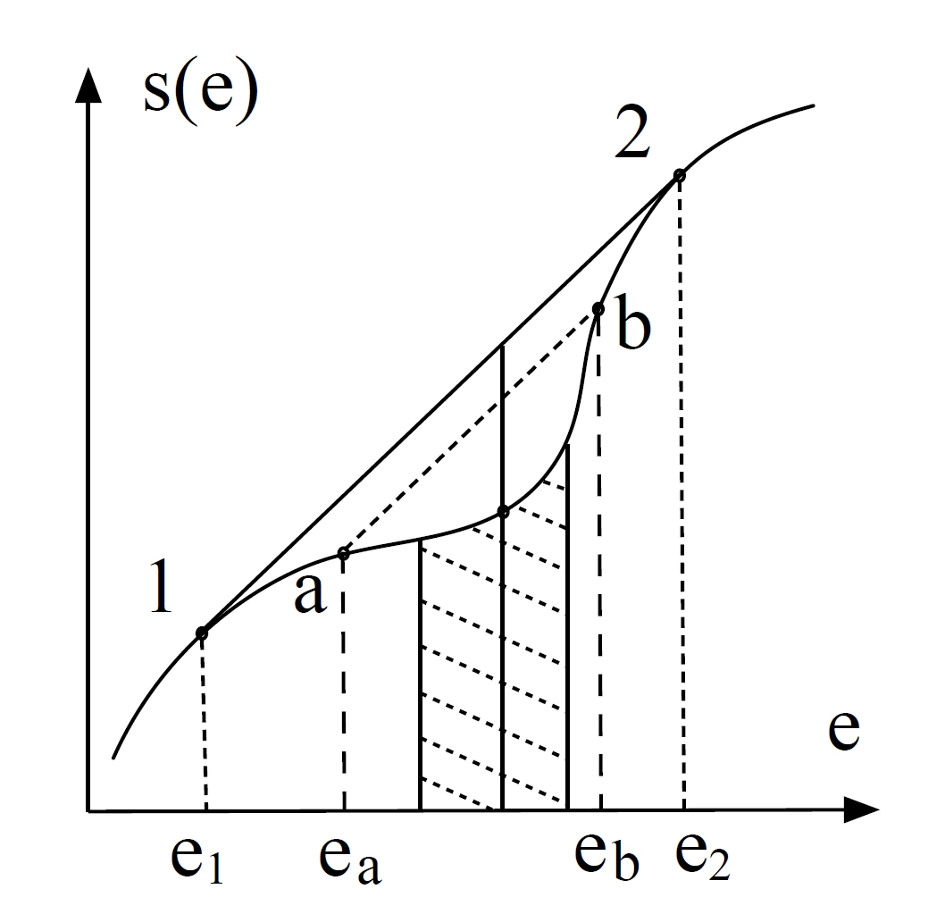
Let’s go back to the curve of entropy.
For any energy
we can achieve higher entropy by forming a mixture of two phases:
- Fraction
in phase (energy , entropy ) - Fraction
in phase (energy , entropy )
The mixture entropy exceeds the homogeneous entropy:
The optimal phases (
The straight line connecting
and must be tangent to at both points This requires equal slopes at
and :
The slope equality implies:
This guarantees thermal equilibrium between the two phases.
Temperature at this point is denoted as
called critical temperature.
Furthermore, we can show chemical equilibrium:
The equilibrium entropy follows the concave hull:
where the mixture entropy is the linear interpolation:
Between
So we can find the capacity divergent:
The apparent contradiction between the microcanonical heat capacity
This divergence eliminates the distinction between positive and negative values -
the pole singularity renders the sign ambiguity physically meaningless.
The “negative”
in the microcanonical ensemble and the strictly positive
converge to identical divergent behavior at the phase transition.
It agrees with our life experiment.
We know that melting and boiling will absorb extra heat while temperature remains unchanged.
According to the definition of capacity,
it is bound to be infinite.
The heat change during the process is called latent heat.
We will clarify more details in the following sections.
We must pay attention to the fact that
the convex curve is a result of state equation,
and the double tangent line is how entropy evolves in reality.
The entropy curve’s convex region arises directly from the system’s fundamental equation of state—this curved path represents all possible homogeneous configurations governed by microscopic interactions. However, this convex segment remains thermodynamically forbidden in physical systems due to its instability. The double tangent line reveals what actually occurs: systems spontaneously undergo phase separation to follow this straight-line path in the entropy-energy plane.
This straight trajectory connects coexisting phases at energies
This geometric duality—curved state equation versus straight phase-transition path—explains why boiling water at 100°C absorbs heat without temperature change: the system evolves along the double tangent line, not the unstable curved entropy path predicted for homogeneous states.
2.8.3 Phase Transition under Canonical Ensemble
Since the conflict has been solved,
we will derive the whole system with canonical ensemble.
Consider a simple fluid (
Pressure is obtained via derivative:
The mechanical stability condition requires:
When this condition is violated in interval
phase separation occurs.
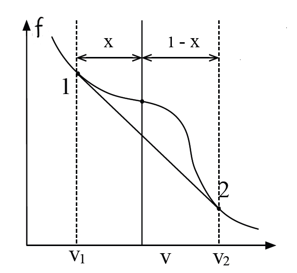
Using the same method,
we find the two points of phase transition via
Transition points satisfy:
where
For
Equilibrium free energy is the convex hull:
We can still derive equlibrium condirtions:
Thermal equilibrium: Same
Mechanical equilibrium:
Chemical equilibrium:
2.8.4 Maxwell Construction
The Helmholtz free energy curve exhibits a concave region within the phase transition interval.
This concavity violates the mechanical stability condition requiring
indicating that homogeneous states in this region are thermodynamically unstable.
The chemical equilibrium condition for coexisting phases is given by:
Using the pressure definition:
we evaluate the integral:
This result is the Maxwell construction,
whose essence is the enforcement of chemical potential equilibrium.
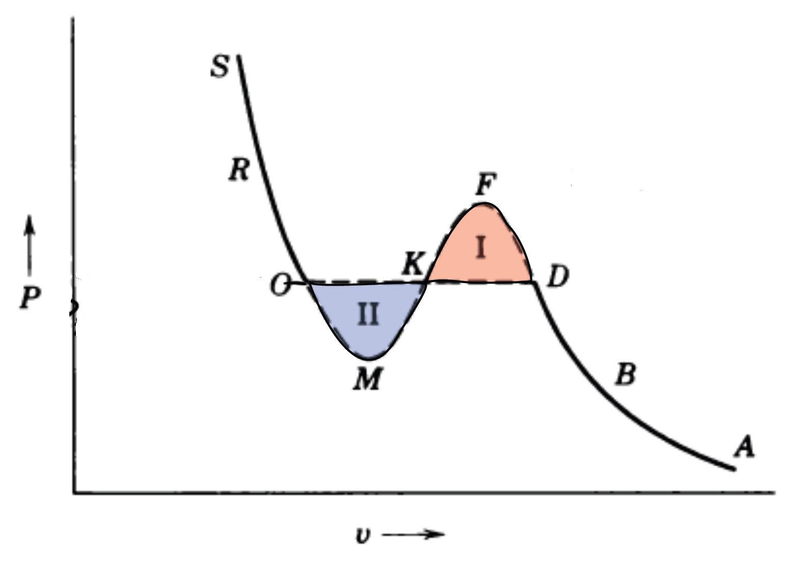
Geometrically,
it requires the area of Region I to equal that of Region II in the figure below:
2.8.5 Latent Heat
During first-order phase transitions like boiling or melting,
systems absorb or release significant energy while maintaining constant temperature—
a phenomenon most familiar when water boils at
and remains at that temperature until fully vaporized.
This hidden energy exchange,
termed latent heat (denoted
breaks or forms molecular bonds rather than increasing thermal motion.
For a system of
the total latent heat is quantified as
where
represents the entropy difference per particle between phases—for example,
vaporizing water requires approximately
Crucially, latent heat equivalently equals the enthalpy difference
expressed as
a relationship arising directly from the equality of chemical potentials
(
The coexistence of phases in the temperature-pressure
(
plane is defined by the chemical potential equality
describing an intersection curve of two surfaces in
elsewhere, the phase with lower
When tracing small displacements along this coexistence curve (
the preservation of chemical equilibrium
where
This equation reveals how coexistence pressures shift with temperature: for most substances,
volume expands during melting or boiling (
resulting in a positive slope (
water, however, exhibits anomalous behavior where ice melting decreases volume
(
producing a negative slope (
that explains why increased pressure melts ice at constant temperature—a principle enabling ice skating.
For water boiling at
the values
indicating substantial pressure sensitivity near phase boundaries.
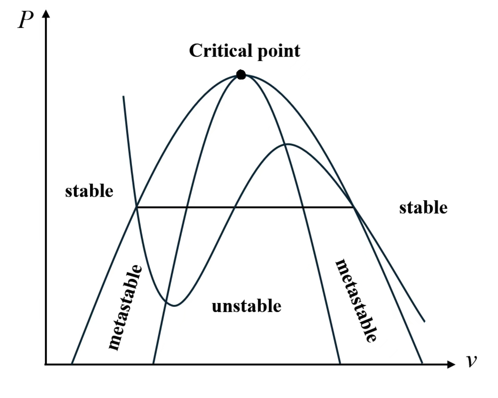
2.8.6 Stable and Metastable
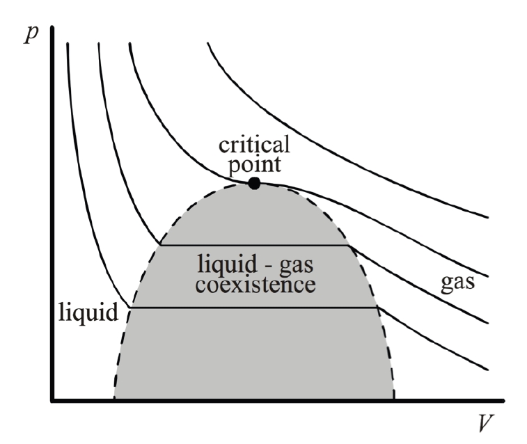
The critical point is the thermodynamic state where distinct liquid and gas phases become indistinguishable,
characterized by:
Critical temperature (
) Critical pressure (
) Critical volume (
)
At this point, liquid-gas coexistence terminates,
surface tension vanishes,
and thermodynamic response functions
(e.g., compressibility
You can see it clearly in the following figure:
Taking Van der Waals gas for example.
It has state equation of
where
For temperatures below
which means there’re concave regions.
This region indicates
The boundary of phase transition is constructed by Maxwell construction.
The critical point is determined by
Solving this for Van der Waals gas, the result is
We need to illustrate the elements in
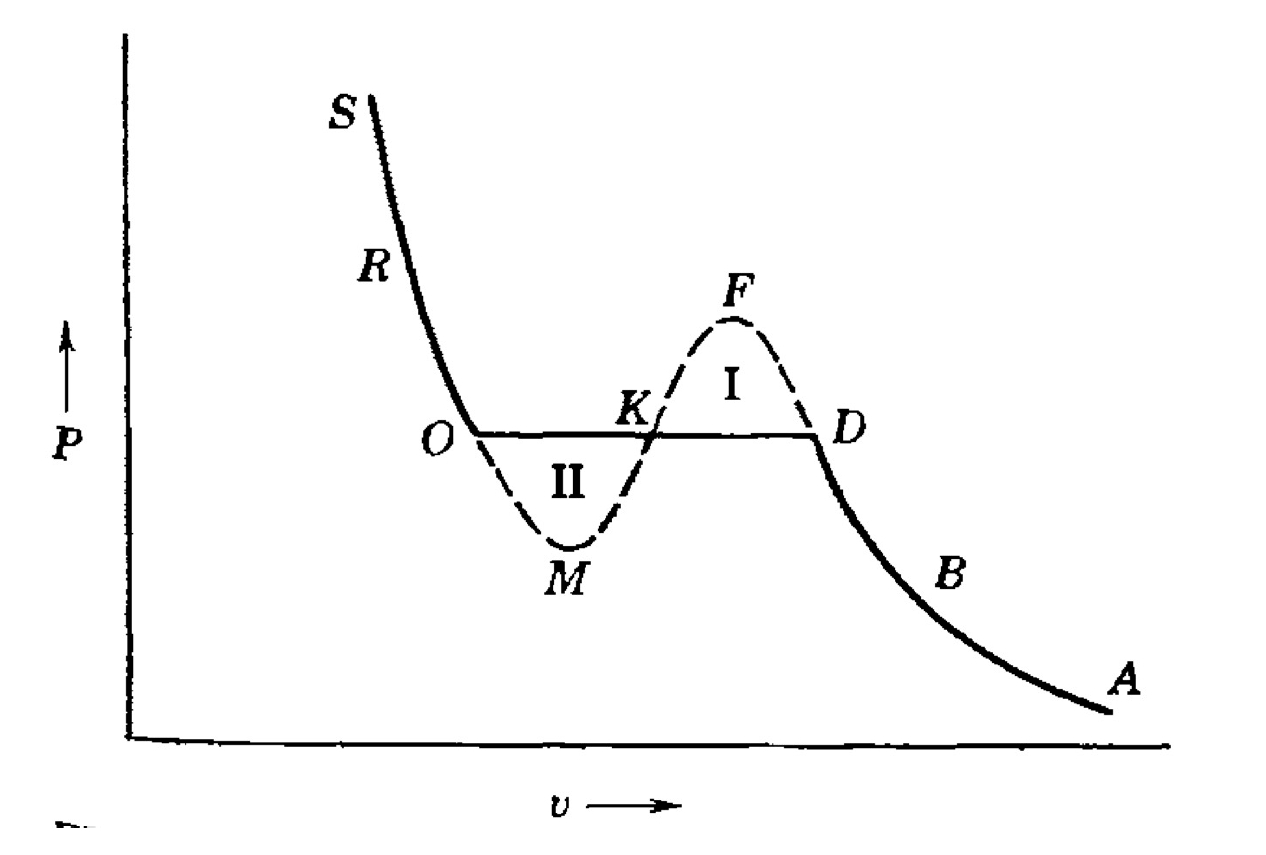
We must relate this figure to the Helmholtz free energy double tangent line.
Point O and D are the phase transitions boundary,
corresponding to the tangent points of
Line OD is the projection of constructed double tangent line.
Curve OMFD is the projection of
Obviously, with temperature growing,
skrewed point M and F gradually converges to their middle point K
and finally merged to one point at critical temperature
What still puzzles us is the meaning of point M and F.
Notice that between M and F is the unstable region we mentioned above.
so M and F is the boundary of instability regions.
The segments OM and FD correspond to metastable states,
where the system resides in a local minimum of the Helmholtz free energy.
These states satisfy local stability conditions
(
but are thermodynamically inferior to the phase-separated state on the Maxwell line.
Classic examples include:
Supercooled water: Liquid persists below
(e.g., down to ) due to kinetic barriers inhibiting ice nucleation. Superheated water: Liquid exists above
(e.g., up to at high pressure) without boiling.
These metastable states are sensitive to perturbations:
Nucleation triggers collapse: Introduction of impurities, vibrations, or density fluctuations drives the system toward the global minimum—spontaneously phase-separating along the Maxwell line OD.
Physical mechanism: Local free energy minima (OM/FD) are separated from the coexistence line (OD) by energy barriers; once overcome, the system releases latent heat and achieves equilibrium via phase separation.
Now we will have to calculate the exact boundary line on
We will use a method called asymptotic expansion.
Still take Van der Waals gas,
To analyze behavior near the critical point, we define reduced variables:
Expanding the Van der Waals equation around the critical point gives:
This governs liquid-gas coexistence for
The coexistence volumes
Equal pressure:
Equal chemical potential:
Maxwell area rule:
Assume asymptotic expansions (square root to avoid pole point):
Combining the equations above and matching orders of
Applying the area condition determines
Thus, the coexistence volumes are:
and the coexistence pressure is:
The derivative defines stability:
The spinodal points
(where
Here is a summary:
Stable liquid:
Stable gas:
Metastable supercooled liquid:
Metastable superheated vapor:
Unstable (spinodal) region:
2.8.7 Gibbs Phase Rule
In this section we will research multi-component systems.
For multi-component systems,
differential equation of energy is expanded to
Gibbs free energy
is especially useful here.
Its differential form is
This equation gives
Commutativity of partial derivatives then leads to
Inspecting formulas above,
we may find a constraint of chemical potential:
So
Now suppose we have a system with
and
Coexisting phases means the two phases have macroscopic, observable boundary.
For example, solid ice, liquid water, soild alcohol are three coexisting phases.
2.8.8 Chemical Reactions
Consider a chemical reaction involving2.9 Second Order Phase Transition
2.9.1 Ising Model
A phase transition occurs when a material’s macroscopic properties change abruptly as an external parameter,
like temperature, is varied.
In a first-order phase transition,
exemplified by phenomena like boiling where density changes suddenly,
specific thermodynamic quantities exhibit a discontinuous jump at the transition point.
Second-order phase transitions,
also termed continuous phase transitions,
present a different picture.
Here, a fundamental physical quantity known as the order parameter is central.
The order parameter quantitatively measures the degree of order or broken symmetry within the material’s structure.
Specifically, the order parameter takes on a non-zero value in the phase exhibiting long-range order,
typically at lower temperatures,
signifying the established order,
such as spontaneous magnetization in a ferromagnet.
As the temperature approaches the critical temperature in a second-order transition,
this order parameter diminishes continuously and smoothly,
finally reaching zero in the disordered, high-temperature phase.
Crucially, while the order parameter itself evolves continuously to zero in a second-order transition,
its derivatives with respect to external parameters like temperature –
quantities such as susceptibility or specific heat –
typically exhibit discontinuities or even diverge at the critical point.
Therefore, the defining characteristic distinguishing first-order from second-order phase transitions
lies in the behavior of the order parameter:
a discontinuous jump signals a first-order transition,
whereas a continuous decrease to zero signifies a second-order transition.
Local alignment: Exchange interactions drive near-perfect parallel alignment of atomic moments within each cell
Spontaneous symmetry breaking: The entire cell spontaneously selects a preferred magnetization direction
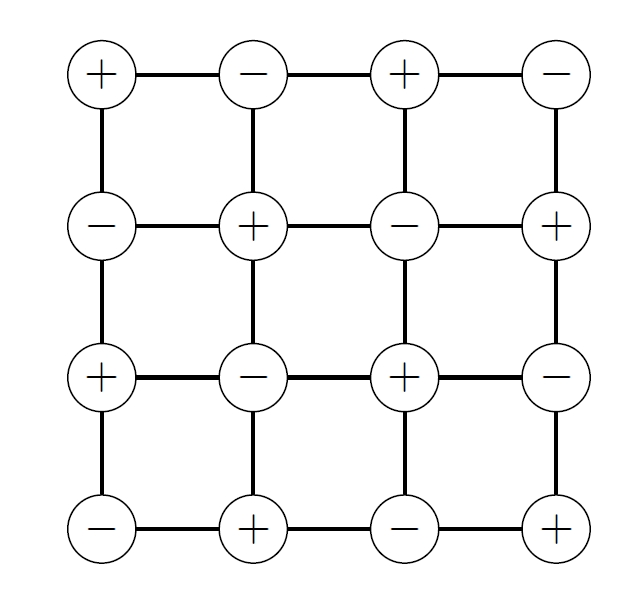
We replace the actual fluctuating interactions on a spin with an effective field generated by the average magnetization of its neighbors.
Based on this assumption, probabilities of each spin are decoupled and become independent. Then the joint distribution becomes simple product of each probabilities:2.9.2 Scaling Hypothesis
In second-order (continuous) phase transitions, the system's symmetry changes, and critical phenomena emerge near the critical point. These phenomena—including power-law divergences, scaling laws, universality, and fractal behavior—arise from the divergence of the correlation lengthA singular (divergent) part: This part diverges or vanishes as a power law at the critical point.
A regular (smooth) part: This part remains finite and non-singular.
The critical exponents are defined by the power-law scaling of the singular parts.
Below are the key power-law relations,
illustrated using the Ising model as an example.
Specific Heat (
): The singular part of the specific heat diverges as when (i.e., as ). For , diverges at ; for , it may exhibit a logarithmic divergence. Order Parameter (
): Below ( ), the spontaneous magnetization (order parameter) vanishes as . This describes how the ordered phase disappears as approaches from below. Susceptibility (
): The magnetic susceptibility (response to an external field) diverges as near . This indicates enhanced response to perturbations at criticality. Critical Isotherm (
at ): At ( ), the magnetization depends on the external field as a power law. A large implies weak response to near criticality. Correlation Function (
): The correlation function describes spatial correlations. The correlation length indicates how far one spin can affect another spin. At criticality ( ), it decays algebraically as , where is the spatial dimension. The exponent quantifies deviations from mean-field decay. Correlation Length (
): The correlation length diverges as near , defining the spatial scale over which fluctuations are correlated. This divergence underpins all critical phenomena.
- Singular part of free energy. Near the critical point, the free
energy
can be decomposed into a smooth part and a singular part. The singular part is assumed to be a generalized homogeneous function of and : is called the scaling function, which is smooth except at Single length scale: Close to the critical point, the correlation
length, becomes the only relevant length scale.
This means that second order transition is because that
near the critical point,
correlation length becomes too large (divergent)
that all microscopic scales are too small compared to the correlation length.
Fisher law:
Rushbrooke law:
Widom law:
Josephson law:
Therefore only two of these exponents are independent.
2.9.3 Landau Free Energy
Let us go back to the Ising HamiltonianFirst, sum over all spin configurations with fixed
. Then sum over all allowed values of
.
saddle point approximation
. Then2.9.4 Landau Theory of Phase Transitions
We define free energy per spin and Landau free energy per spin:When
, , and we can ignore the quartic term in the Landau free energy because . The minimum occurs at , and substituting back gives: Evidently, and are respectively the regular part and the singular part of the free energy. We need to cast the singular free energy into the scaling form. The equation above gives . To balance coefficient, This gives However, defines the behavior of . From the exact form of , when , sigular part vanishes. Then we can only have one solution: Note that converges under such parameters configuration. This is in fact the limitations of Landau's theory. When
, from the analysis above, is always the regular part of the free energy. We may therefore ignore it in the Legendre transform and focus directly on the singular free energy. For , the singular free energy is derived by minimizing: To extract the scaling form, rescale the variables. Define the dimensionless magnetization and field: Substituting into the free energy expression gives: where is a dimensionless function determined by the dimensionless minimization problem. This recovers the scaling form: confirming the critical exponents: Other exponents can also be calculated by Landau's function. Spontaneous magnetization exponent
: At and , minimization of the Landau free energy gives: Thus, . Critical isotherm exponent
: At , minimization yields: Hence, . Susceptibility exponent
: For ( ), the linear response gives: Thus, . Correlation length exponent
and correlation function exponent : Using the Gaussian approximation of the Landau-Ginzburg functional: The correlation function satisfies: with solution: This implies . The short-distance behavior corresponds to (since implies ). Verification via Fisher relation:
The consistency is confirmed by:Summary of mean-field exponents: All critical exponents in Landau theory are:
These satisfy the scaling relations and are exact for spatial dimensions .
Part III. Quantum Statistical Mechanics
3.1 Fermions and Bosons
3.1.1 Fundamental Properties
Fermions—encompassing electrons, protons, neutrons, and quarks—are quantum particles with
half-integer spin
whose wavefunctions exhibit antisymmetry under particle exchange.
This defining property arises from the spin-statistics theorem and fundamentally shapes their behavior:
- Fermionic antisymmetry: The wavefunction reverses sign when any two particles are exchanged:
- Pauli exclusion principle: Fermions resist occupying identical quantum states, leading to spatial exclusion and degeneracy pressure in neutron stars and white dwarfs.
Bosons—including photons, gluons, and Higgs bosons—possess integer spin
and exhibit symmetric wavefunctions under particle exchange:
- Bosonic symmetry: The wavefunction remains invariant under particle exchange:
- Bose enhancement: Multiple bosons congregate in low-energy states, enabling phenomena like superconductivity and Bose-Einstein condensation.
Quantum particles also obey principle of indistinguishability
fundamentally distinguishes quantum statistics from classical mechanics.
While classical particles maintain identity through trajectories,
quantum particles lose individuality—their wavefunctions coalesce into collective states.
The permutation operator
and
Crucially in 3+1 dimensions,
requiring physical states to transform as:
This phase constraint crystallizes the spin-statistics theorem:
Fermions (
) inhabit antisymmetric wavefunctions Bosons (
) populate symmetric wavefunctions
If there’re two particles in one system,
fermions are constrained by Pauli exclusion principle while bosons don’t:
Fermions:
This state vanishes when
Bosons:
When
And now we expand the system to
The whole state space becomes products of
called Fock space:
In this Fock space, joint state of all particles
can be represented as derminant or permanent.
For fermions:
The determinant’s antisymmetry ensures wavefunction sign-flips under particle exchange while automatically enforcing exclusion when states coincide.
For bosons:
Summing over all permutations
This symmetry dichotomy orchestrates quantum many-body phenomena—from the stability of matter enforced by fermionic exclusion to the coherent quantum phases enabled by bosonic condensation.
3.1.2 Second Quantization
Suppose we have six particles distributed among single-particle states labeled by momentum or energy eigenstates
Imagine:
Particle 1 in state
Particle 2,3 in state
Particle 4,5,6 in state
The corresponding product state is:
and we must then symmetrize (for bosons) or antisymmetrize (for fermions)
the product state, which is tedious and cumbersome.
However, at the end of this process, we only care about the number
of particles in each single-particle state.
In this case, we combine the same states and denote only occupation numbers:
where
For example, the configuration above will be denotes as
For bosons,
However, fermions must not violate Pauli.
So
3.1.3 Creation and Annihilation Operators
We are now ready to introduce the natural operators that act on these states ( |n_1, n_2, \ldots \rangle : ) creation and annihilation operators. These operators do exactly what their names suggest:
Their action on the occupation number basis is defined as follows:
These definitions ensure the proper normalization of states and preserve the orthonormality of the Fock basis.
The algebra of these operators depends on the statistics of the particles. Traditionally we use
For bosons:
For fermions:
Here,
and
We further define number operators:
To verify, just operate this operator on a state
you will finally get a eigenvalue of
We can easily show the following commutation relations:
- For Bosons:
- For Fermions:
These operators provide a powerful and elegant language for quantum many-body systems. They:
Simplify the construction of many-body states and operators
Encode particle statistics algebraically
Constitute the foundation for quantum field theory and quantum many-body theory
For example, consider the operator:
which is entirely natural in the second quantized language.
It is a linear operator on Fock space,
and when applied to the vacuum,
it yields a valid physical state:
We can use creation operators to construct the occupation number basis
states from the vacuum state:
3.2 Free Fermi Gas
3.2.1 Thermodynamic Properties
For a macroscopic free Fermi gas, the vast number of particles necessitates the use of second quantization to represent the system's state; this formalism inherently incorporates de Broglie's wave-particle duality, where particles exhibit both wave-like character (plane waves) and granularity. To determine the total energy of this non-interacting gas, we use the second-quantized HamiltonianThis is called the Fermi-Dirac distribution.
Furthermore, we can obtain the grand canonical potentialThe average particle number
: The internal energy
: The pressure
:
3.2.2 Density of States (DOS)
In the thermodynamic limit, where the volumeWith the density of states we can rewrite the thermodynamic quantities:
Grand potential
Particle number
Internal energy
3.2.3 Zero Temperature Limit
When the temperature approaches 0, the Fermi-Dirac distribution function reduces to a unit-step function about energy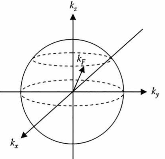
3.2.4 Low Temperature Sommerfeld Expansion
At low but finite temperaturesBuilding upon the Sommerfeld expansion technique, we now systematically examine how key thermodynamic quantities of the degenerate Fermi gas evolve at low temperatures. The expansion provides a powerful framework for calculating precise temperature-dependent corrections to zero-temperature behavior.
Chemical Potential
The fundamental connection between particle number and chemical potential emerges from the density of states and Fermi-Dirac distribution:which simplifies to the constraint equation: Applying the Sommerfeld expansion with yields: Solving perturbatively by writing and expanding in small and gives the chemical potential's temperature dependence: This reveals that decreases quadratically from with increasing temperature, reflecting thermal excitation of fermions just below the Fermi surface. Internal Energy
The internal energy expression:is evaluated using in the Sommerfeld expansion: Substituting the chemical potential from above and re-expanding in produces: The quadratic increase in with temperature contrasts sharply with classical gases, arising from Pauli blocking that restricts excitations to a thin shell near . Pressure and Compressibility
Using the relationfrom the grand potential, pressure inherits the temperature dependence of internal energy: The isothermal compressibility then follows from its thermodynamic definition: Differentiating while noting yields: This shows compressibility decreases with temperature, indicating the gas becomes stiffer as thermal excitations populate states above the Fermi surface.
3.3 Free Bose Gas
3.3.1 Thermodynamic Properties
In this lecture, we study a system of non-interacting massive bosonic particles confined in a volumeOur research path is the same as that of fermions.
Still, in grand canonical ensembleGrand potential
It is instructive to write as a product of infinitely many grand canonical partition functions for one single-particle state systems: Similarly, the grand potential can be written as the sum: These results tell us that the Bose gas can be understood as an independent sum of infinitely many small open systems. These small open systems are in contact with the same bath with temperature and chemical potential . Particle number
This is known as Bose-Einstein distribution.
We also have
3.3.2 High Temperature Limit
At high temperatures or low densities, quantum gases behave classically, with quantum statistical effects appearing as small corrections. The key parameter governing these corrections is the degeneracy parameter3.3.3 Bose-Einstein Condensation
Let's go back to the Bose-Einstein distribution.We consider it as only the particles of excited states instead of all bosons, and bosons have finite excited states. When the particles exceeds the upper bound of excited states number, no matter the energy, the exceeded part must be filled in the ground state. They condensed in the ground state and do not contribute to the property of the entire system. This phenomenon is called Bose-Einstein condensation.
Under this perspective, we can reinterpret the equations above:Because of the condensation,
the system is divided into two phases:
Condensate: A macroscopic number of particles occupy the ground state
. These particles have zero kinetic energy and zero mo- mentum. As a result, they contribute nothing to the energy, pressure, or entropy of the system. Thermal Cloud: All other particles are distributed among excited states with
, described by the usual Bose-Einstein distribu- tion with . These particles determine all thermodynamic properties energy, pressure, and heat capacity.
- Isothermal Compressibility
The thermal cloud exhibits critical behavior near
. The isothermal compressibility quantifies its response to pressure changes at fixed temperature: With fixed, variations in and arise solely from changes in via : Using the identity , these become: In logarithmic form ( ): The ratio yields : where is fixed by . As , and diverges while remains finite. Consequently, diverges:
3.4 Trapped in a Potential
The behavior of quantum gases confined in external potentials exhibits fundamental differences from free-space systems, with harmonic traps3.5 Massless Quantum Gas
3.5.1 Density States
Massless bosonic particles such as photons and phonons exhibit a linear dispersion relation3.5.2 Blackbody Radiation
The electromagnetic field in thermal equilibrium is modeled as a gas of non-interacting photons with zero chemical potential. Each mode of frequency3.5.3 Lattice Vibration
In solids, lattice vibrations are quantized as phonons with linear dispersionAt high temperatures (
), (Dulong-Petit law). At low temperatures (
), due to phonon modes behaving as massless bosons. In metals, low-temperature specific heat combines electronic and phonon contributions: , where probes the Fermi surface and reflects phonon properties. The Debye model succeeds by capturing the finite mode density and linear dispersion of acoustic phonons, while Einstein’s model (single-frequency oscillators) fails at low due to its exponential suppression of .
References:
[1] 李椿, 章立源, 钱尚武, 热学, 第三版. 北京: 高等教育出版社, 2015.
Note: Part of the mathematical formatting and structural organization of this article were assisted by AI models